
H2M L15 Q2: Interactive Exploration of Random Variables and Linear Programming
Loading the math board and drawing, please wait…
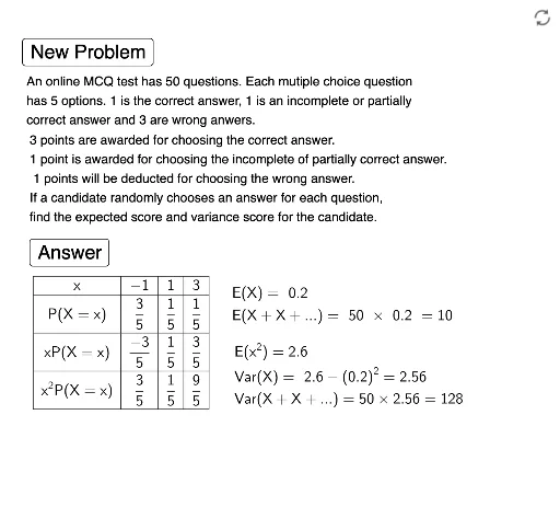
This GeoGebra example dynamically demonstrates the interplay among random variables, variance, volume, rhombus geometry, coordinates, and linear programming, with a scatter plot visualizing data distribution. Core mathematical concepts include generation of random variables and their statistical properties (e.g., variance), feasible regions and objective function optimization in linear programming, and representation of geometric shapes (rhombus) in a coordinate system. Construction highlights: uses Random and RandomElement commands to generate random data, Sequence and Sum to build sequences and statistics, Join and TableText to organize data tables; interface includes buttons (button1, button2) for triggering random updates, multiple text objects (text1 to text6) displaying computed results, and variables (o, a, b, c, e, f, vx, etc.) storing intermediate values. Suitable for high school or early college students to understand the combination of random simulation and linear programming, and also useful for teachers as a classroom demonstration or for student self-exploration.
GeoGebra Commands & Parameters
Random(4, 5) → bRandomElement({1, 2}) → cSequence((Element[l1, i] * Element[l2, i]), i, 1, 3) → l3Sum(l3) → exJoin({{"x P(X=x)"}, Sequence[FractionText[Element[l3, i]], i, 1, 3]}) → l7TableText(l1, l2, l3) → text3Join({{"x"}, Sequence[FractionText[Element[l1, i]], i, 1, 3]}) → l5Join({{"P(X=x)"}, Sequence[FractionText[Element[l2, i]], i, 1, 3]}) → l6Sequence((Element[l1, i]^(2) * Element[l2, i]), i, 1, 3) → l4Join({{"x^2 P(X=x)"}, Sequence[FractionText[Element[l4, i]], i, 1, 3]}) → l8TableText(l5, l6, l7, l8, "c |_") → text4Sum(l4) → e
AI Drawing Prompt Reference
Create a scatter plot to show the probability distribution and variance of a random variable. Generate random values for x and calculate their probability distribution, variance, and x^2 probability distribution. Use these data to create a table displaying the values of x, P(X=x), and x^2 P(X=x). Draw the feasible region and objective function to illustrate a linear programming problem. Plot a rhombus in the coordinate system to show its geometric properties. Generate random data and update the graph, triggering random updates with buttons.
The prompt above was compiled from the original drawing commands and is for reference only.