
Limit Laws Demonstration
Loading the math board and drawing, please wait…
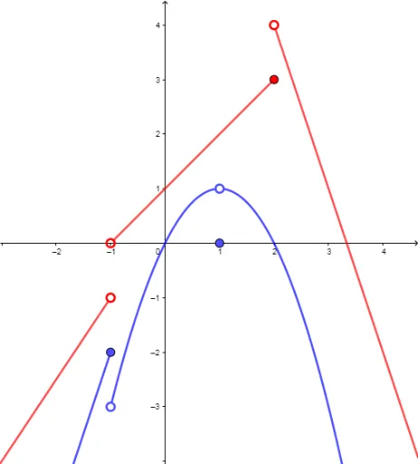
This example demonstrates the application of Limit Laws in function graphs by dynamically adjusting parameters to observe limit value changes. Core math concepts include limits, functions, natural numbers, scatter plots, and median values. GeoGebra commands like f, g, h, sliders, and limit1 are used to construct function and limit animations. Suitable for high school and university beginners studying calculus limits, ideal for teaching demonstrations and concept understanding.
GeoGebra Commands & Parameters
f(x) = If[-0.98 ≤ x < 0.93, (-(x - 1)^(2)) + 1](1, 1)(-1, -3)g(x) = If[x ≥ 1.08, (-(x - 1)^(2)) + 1]h(x) = If[x ≤ -1, (3 * x) + 1](-1, -2)(1, 0)p(x) = If[x < -1.05, (1.5 * x) + 0.5]q(x) = If[-0.95 < x < 2, x + 1]r(x) = If[x > 2.03, (-3 * x) + 10](-1, 0)(-1, -1)(2, 3)(2, 4)truefalsefalsefalseNumeric Example(1)Numeric slider(0.99)(slider - 2, (3 * (slider - 2)) + 1)falsefalsefalsefalsefalsefalsefalsefalse(slider - 2, (1.5 * (slider - 2)) + 0.5)((-slider), (-((-slider) - 1)^(2)) + 1)((-slider), (-slider) + 1)(slider - 1, (-(slider - 2)^(2)) + 1)(slider - 1, slider)((-slider) + 1, (-((-slider))^(2)) + 1)((-slider) + 1, (-slider) + 2)(slider, (-(slider - 1)^(2)) + 1)(slider, slider + 1)((-slider) + 2, (-((-slider) + 1)^(2)) + 1)((-slider) + 2, (-slider) + 3)(slider + 1, slider + 2)((-slider) + 3, (-((-slider) + 2)^(2)) + 1)(slider + 1, (-slider^(2)) + 1)((-slider) + 3, (-3 * ((-slider) + 3)) + 10)false