
Left Rectangle Approximation for Area Under a Curve
Loading the math board and drawing, please wait…
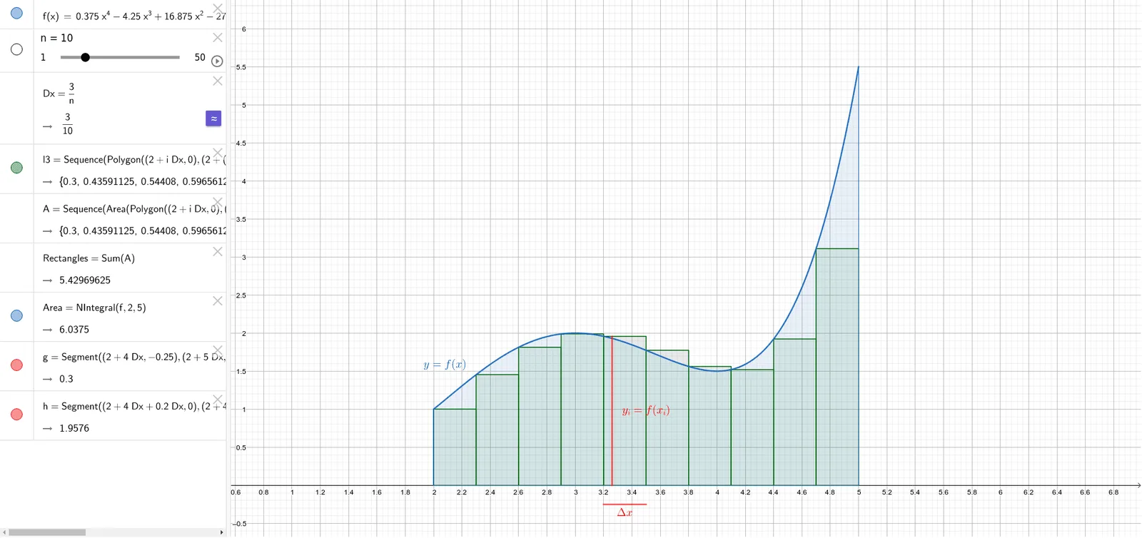
This example demonstrates the left rectangle approximation method for estimating the area under a curve. Key mathematical concepts include integration, rectangle area calculation, and function graphs. Using GeoGebra commands such as Sequence, Sum, NIntegral, and Segment, a series of rectangles are constructed to approximate the area under the curve. Suitable for high school mathematics education and learning integration concepts.
GeoGebra Commands & Parameters
Sequence(Polygon[(2 + (i * Dx), 0), (2 + ((i + 1) * Dx), 0), (2 + ((i + 1) * Dx), f(2 + (i * Dx))), (2 + (i * Dx), f(2 + (i * Dx)))], i, 0, n - 1) → l3Sequence(Area[Polygon[(2 + (i * Dx), 0), (2 + ((i + 1) * Dx), 0), (2 + ((i + 1) * Dx), f(2 + (i * Dx))), (2 + (i * Dx), f(2 + (i * Dx)))]], i, 0, n - 1) → ASum(A) → RectanglesNIntegral(f, 2, 5) → AreaSegment((2 + (4 * Dx), -0.25), (2 + (5 * Dx), -0.25)) → gSegment((2 + (4 * Dx) + (0.2 * Dx), 0), (2 + (4.2 * Dx), f(2 + (4 * Dx)))) → h