Lagrange Multiplier

Loading the math board and drawing, please wait…

2020-07-09 19:45

Calculus Derivative Optimization

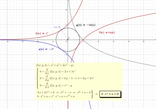
This example demonstrates the Lagrange multiplier method for solving optimization problems with constraints. Key mathematical concepts include functions, derivatives, and extrema. Using GeoGebra commands such as Intersect, Point, and Circle, the construction process involves creating essential geometric objects. Suitable for high school mathematics education, particularly in calculus and optimization.

GeoGebra Commands & Parameters

Intersect(xAxis, yAxis) → A
Point(h) → B
Circle(A, B) → c
LaTeX(h, true, true) → texto1
Segment(A, B) → i
LaTeX(g, true, true) → texto3
LaTeX(p, true, true) → texto5
LaTeX(f, true, true) → texto6

AI Drawing Prompt Reference

Draw a diagram illustrating the Lagrange multiplier method for constrained optimization. Start with coordinate axes and mark the origin as a fixed point. Choose a moving point on a curve, then draw a circle centered at the origin passing through that point. Connect the origin and the moving point with a line segment. Display the formulas for the objective function, the constraint, and related expressions as text labels near the diagram. The overall layout shows the geometric relationship among the curve, circle, segment, and formula annotations to demonstrate the extremum-finding process under constraints.

The prompt above was compiled from the original drawing commands and is for reference only.