Key Features of Trigonometric Graphs (Part 1)

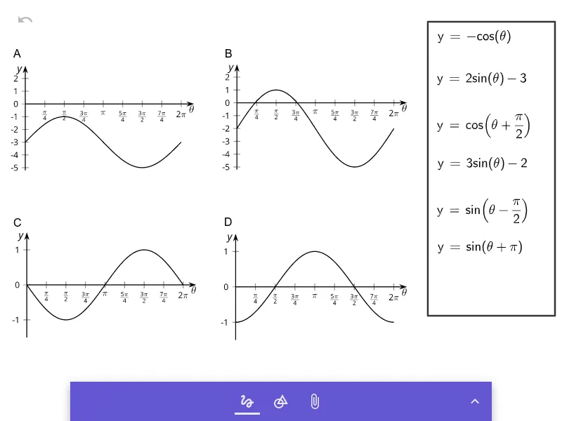
This GeoGebra lesson example demonstrates the main geometric features of trigonometric function graphs and how they change under parameter variations. The central math concepts include periodicity, amplitude, midline shifts, phase changes, and frequency effects (how the wave stretches/compresses horizontally). It focuses on interpreting the curve within one period and relating notable points and bounds to parameters in models such as y = A·sin(B(x−C)) + D or y = A·cos(B(x−C)) + D. Construction-wise, the provided construction summary is empty, so the typical implementation relies on defining the trigonometric function with parameters and graphing it in GeoGebra, then visualizing how A, B, C, and D affect amplitude, cycle length, horizontal positioning, and vertical shift—often using interactive inputs (e.g., sliders) to compare outcomes. Suitable for middle/high school function instruction and for early university precalculus/trigonometry graphing practice.