
Investigating Cosine Graph Transformations
Loading the math board and drawing, please wait…
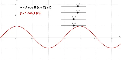
This GeoGebra example demonstrates how the cosine graph changes under common transformations such as horizontal/vertical shifts and related parameter adjustments, emphasizing the geometric correspondence between the original and transformed curves. It focuses on key ideas in trigonometry and function graphing: periodicity of cosine, the role of amplitude and phase, and how translation affects the graph’s shape and location. A calculus-oriented viewpoint is also incorporated by connecting the visual behavior of the curve to derivative-related reasoning. Construction is organized around GeoGebra objects f and g (the cosine-based functions), points/parameters A, B, C, and D to define reference positions, and text1/text2 to label important features for comparison. The interactive setup makes it suitable for secondary advanced learners through pre-college level, as well as for guided classroom exploration and graph transformation practice.
GeoGebra Commands & Parameters
f(x) = cos(x)Numeric A(1)Numeric B(1)Numeric D(0)Numeric C(0)g(x) = (A * cos((B * (x + C)))) + D
AI Drawing Prompt Reference
Draw the graph of a cosine function and its transformations under horizontal and vertical shifts, as well as parameter adjustments. Start by plotting the basic cosine curve, then draw the transformed cosine curve based on the adjusted parameter values. Mark several key points in the graph to compare the positions of the original and transformed curves, and add text labels to highlight important transformation features.
The prompt above was compiled from the original drawing commands and is for reference only.