
Introduction to Parametric Equations by Tatiana Yudovina
Loading the math board and drawing, please wait…
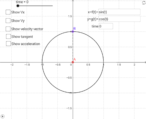
This example demonstrates the basic concepts of parametric equations using vectors and time parameters to represent curves. Key mathematical concepts include parametric equations, vectors, and derivatives. It utilizes commands like CurveCartesian, Vector, and Derivative in GeoGebra. Suitable for high school math education and students learning parametric equations.
GeoGebra Commands & Parameters
CurveCartesian(f(t), g(t), t, 0, 49) → a_1Vector((0, 0), a_1(time)) → uDerivative(f) → dfdtDerivative(g) → dgdtVector((dfdt(time), dgdt(time))) → velVector((f(time), g(time)), (f(time) + dfdt(time), g(time) + dgdt(time))) → vVector((f(time), g(time)), (f(time) + dfdt(time), g(time))) → vxVector((f(time), g(time)), (f(time), g(time) + dgdt(time))) → vyVector((0, g(time)), (0, g(time) + dgdt(time))) → wVector((f(time), 0), (f(time) + dfdt(time), 0)) → bCurveCartesian(dfdt(t), dgdt(t), t, 0, 49) → cTextfield(f) → InputBox1Textfield(g) → InputBox2Segment(C, A) → hSegment(C, B) → iTextfield(time) → InputBox3Tangent(C, a_1) → jDerivative(dfdt, t) → axDerivative(dgdt, t) → ayVector((f(time), g(time)), (f(time) + ax(time), g(time) + ay(time))) → avector
AI Drawing Prompt Reference
Draw a parametric curve and represent its position, velocity, and acceleration using vectors. Start by plotting the curve defined by parametric equations, then draw vectors from the origin to show the curve's position at various points. Calculate and display velocity and acceleration vectors. Use distinct colors for position, velocity, and acceleration vectors, and label key points. Finally, draw the tangent line and the derivative curve.
The prompt above was compiled from the original drawing commands and is for reference only.