Intersection of Parametric and Implicit Curves in R^2

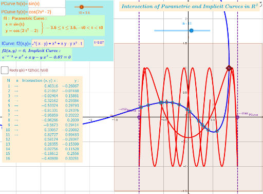
① This example demonstrates how to dynamically find all intersection points between a parametric curve and an implicit curve in the 2D plane using GeoGebra, with the points clearly displayed. ② Core mathematical concepts include parametric equations, implicit equations, solving curve intersections, numerical root-finding, and geometric construction. ③ Construction highlights: the ImplicitCurve command defines the implicit curve, CurveCartesian creates the parametric curve, Zip with Length and Element processes the list of intersection points, OrthogonalLine constructs auxiliary perpendicular lines, Textfield and InputBox provide interactive input, Polygon and TableText are used for visualization and data display, and sliders (t0, t_max, t_min, dt2) control the parameter range. ④ Suitable for upper high school or early university courses in analytic geometry, calculus, or computer-assisted mathematics, and for teachers demonstrating numerical methods for curve intersections.