
Intersection of a Cone and a Cube
Loading the math board and drawing, please wait…
In collections
intersection: surface-surface, curve-curve
intersection: surface-surface, curve-curve
intersection: surface-surface, curve-curve
intersection: surface-surface, curve-curve
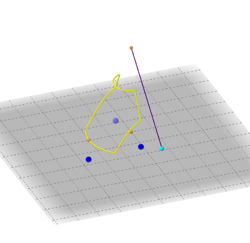
This example demonstrates the intersection lines of a cone and a cube. Key mathematical concepts include solid geometry, distance, and midpoint. Using GeoGebra commands such as Circle, OrthogonalLine, Cone, Cube, and Intersect, the changing intersection lines can be observed. Suitable for high school geometry learners and teachers.
GeoGebra Commands & Parameters
Circle(A, B) → cOrthogonalLine(A, xOyPlane) → fPoint(f) → DCone(c, Distance[A, D]) → b, d, ePoint(c) → FSegment(D, F) → gDistance(A, B) → jMidpoint(A, B) → EPoint(Circle[G, Distance[C, G], Segment[C, G]]) → HCube(C, G, H) → a, I, caraHIML, caraJKLM, arestaCI, arestaCG, arestaGH, arestaHI, arestaCJ, arestaIM, arestaJM, arestaJK, J, arestaGK, arestaKL, arestaHL, arestaLM, K, L, M, caraCGHI, caraCIMJ, caraCGKJ, caraGHLKIntersect(g, caraJKLM) → NIntersect(g, caraHIML) → OIntersect(g, caraGHLK) → PIntersect(g, caraCIMJ) → QIntersect(g, caraCGKJ) → SIntersect(g, caraCGHI) → TLocus(N, F) → LlocGeomètric1Locus(O, F) → LlocGeomètric2Locus(P, F) → LlocGeomètric3Locus(Q, F) → LlocGeomètric4Locus(S, F) → LlocGeomètric5Locus(T, F) → LlocGeomètric6