
Interpreting Correlation - the effect of rescaling
Loading the math board and drawing, please wait…
In collections
Resources for New A-level Maths Spec
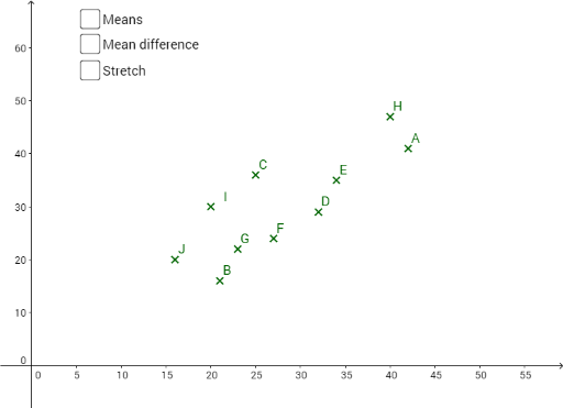
This example demonstrates how rescaling data on separate or both axes affects the correlation coefficient. Key math concepts include correlation, data rescaling, and their impact on scatter plots. It uses GeoGebra commands like Element, Sum, Mean, PointLineSegment, Zip, Sequence, Length, Covariance and objects such as h, d, e, f, J, I, H, G, F, E, D, C, B, A, list2, E2, list1, C2, B2, C5, B5, C11, B11, C10, B10, C9, B9, C8, B8, C7, B7, C6, B6, C4, B4, C3, B3, A1, B1, C1. Suitable for high school students learning the effects of data rescaling on statistical analysis.
GeoGebra Commands & Parameters
Element(list2, 1) → E2Sum(H2:H11) → H12Element(list1, 1) → D2Element(list1, 3) → D4Element(list1, 4) → D5Element(list1, 5) → D6Element(list1, 6) → D7Element(list1, 7) → D8Element(list1, 8) → D9Element(list1, 9) → D10Element(list1, 10) → D11Element(list2, 2) → E3Element(list2, 3) → E4Element(list2, 4) → E5Element(list2, 5) → E6Element(list2, 6) → E7Element(list2, 7) → E8Element(list2, 8) → E9Element(list2, 9) → E10Element(list2, 10) → E11Mean(D2:D11) → D12Mean(E2:E11) → E12PointLineSegment(b, J) → gPointLineSegment(b, F) → iPointLineSegment(b, H) → kPointLineSegment(b, G) → lPointLineSegment(b, E) → mPointLineSegment(b, D) → nPointLineSegment(b, I) → pPointLineSegment(b, C) → qPointLineSegment(b, B) → rPointLineSegment(b, A) → sPointLineSegment(c, E) → tPointLineSegment(c, H) → a_1PointLineSegment(c, F) → b_1PointLineSegment(c, G) → c_1PointLineSegment(c, J) → d_1PointLineSegment(c, I) → e_1PointLineSegment(c, D) → f_1PointLineSegment(c, C) → g_1PointLineSegment(c, B) → h_1PointLineSegment(c, A) → i_1Zip((a, b), a, list1, b, list2) → list3Sequence(If[(x(Element[list3, i]) < Mean[list1]) ∧ (y(Element[list3, i]) < Mean[list2]), ((x(Element[list3, i]) - Mean[list1]) * (y(Element[list3, i]) - Mean[list2])), 0], i, 1, Length[list1]) → list4Sequence(If[(x(Element[list3, i]) > Mean[list1]) ∧ (y(Element[list3, i]) > Mean[list2]), ((x(Element[list3, i]) - Mean[list1]) * (y(Element[list3, i]) - Mean[list2])), 0], i, 1, Length[list1]) → list5Sequence(If[(x(Element[list3, i]) < Mean[list1]) ∧ (y(Element[list3, i]) > Mean[list2]), ((x(Element[list3, i]) - Mean[list1]) * (y(Element[list3, i]) - Mean[list2])), 0], i, 1, Length[list1]) → list6Sequence(If[(x(Element[list3, i]) > Mean[list1]) ∧ (y(Element[list3, i]) < Mean[list2]), ((x(Element[list3, i]) - Mean[list1]) * (y(Element[list3, i]) - Mean[list2])), 0], i, 1, Length[list1]) → list7Element(list1, 2) → D3Length(H2:H11) → H13Covariance(list3) → a
AI Drawing Prompt Reference
Draw scatter plots for two sets of data, showing the mean on both axes, and connect the mean points to the data points with line segments of different colors to visualize the changes in data center. First, plot the scatter plots of the original data sets, then calculate and mark the mean points for each set. Next, connect each data point to the mean points with line segments of different colors, representing the deviation of data points from the mean. Finally, adjust the scaling of the data on the horizontal and vertical axes using a slider to observe the changes in the scatter plots and connecting line segments, as well as the movement of the mean points.
The prompt above was compiled from the original drawing commands and is for reference only.