
Interactive Polygonal Sinusoids
Loading the math board and drawing, please wait…
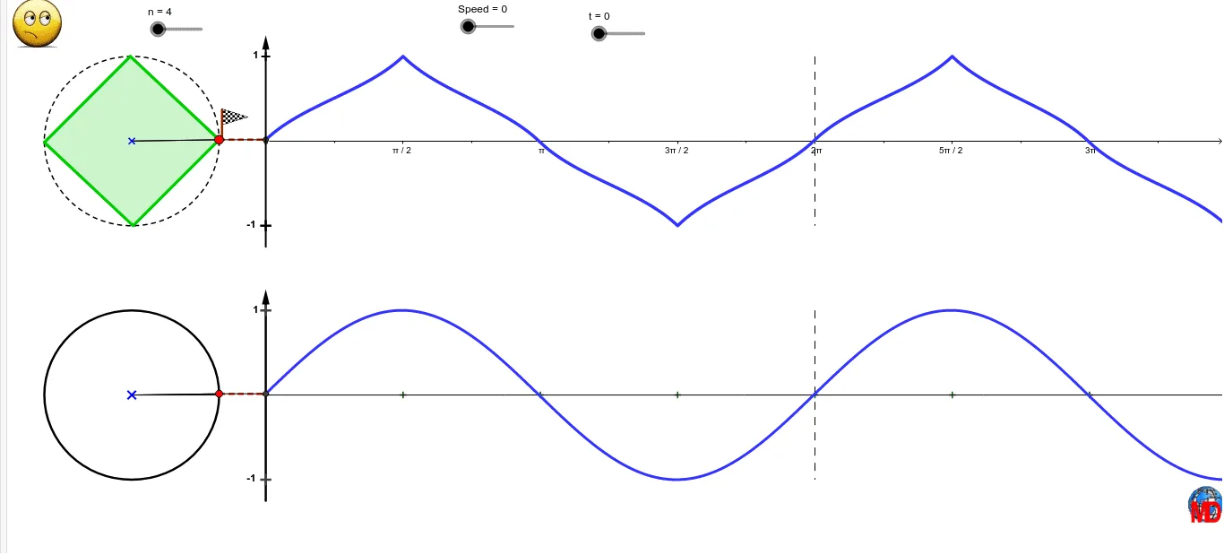
This example demonstrates the dynamic changes of interactive polygonal sinusoids. It involves core concepts of trigonometry and stochastic processes. Using GeoGebra commands such as Circle, Point, Rotate, Segment, Polygon, etc., a series of polygons are constructed and their sinusoidal curves are observed. Suitable for high school mathematics teaching and learning, particularly for trigonometry and geometric construction.
GeoGebra Commands & Parameters
Circle(A, 1) → cPoint(c) → BRotate(B, t, A) → B'Segment(A, B') → gPolygon(B, Rotate[B, (2 * π / n), A], n) → poly1, a, p, q, r, s, a_1, b_1, c_1, d_1, e_1, f_1, b, g_1, h_1, i_1, j_1, k_1, l_1, m_1, q_1, r_1, s_1, d, t_1, C, H, I, J, K, L, M, N, O, h, P, Q, R, S, T, U, V, W, Z, A_1, i, B_1, C_1, D_1, E_1, F_1, G_1, H_1, I_1, J_1, j, k, l, mIntersect(g, poly1) → DPoint(poly1) → EAngle(B, A, D) → αSegment(A, D) → eLocus(G, t) → lieu2Segment(D, G) → fSegment(A, B) → n_1Segment(F, G) → p_1Segment((6.283185307179586, 1), (6.283185307179586, -1)) → a_2Segment(B, K_1) → b_2Circle(N_1, 1) → c_2Point(c_2) → CCPolygon(CC, Rotate[CC, 0.12566370614359174, N_1], 50) → poly2, d_2, m_2, n_2, p_2, q_2, r_2, s_2, t_2, a_3, b_3, c_3, e_2, d_3, e_3, f_3, g_3, h_3, i_3, j_3, k_3, l_3, m_3, f_2, n_3, p_3, q_3, r_3, s_3, t_3, a_4, b_4, c_4, d_4, g_2, e_4, f_4, g_4, h_4, i_4, j_4, k_4, l_4, m_4, n_4, h_2, p_4, O_1, P_1, Q_1, R_1, S_1, T_1, U_1, V_1, W_1, i_2, Z_1, A_2, B_2, C_2, D_2, E_2, F_2, G_2, H_2, I_2, j_2, J_2, K_2, L_2, M_2, N_2, O_2, P_2, Q_2, R_2, S_2, k_2, T_2, U_2, V_2, W_2, Z_2, A_3, B_3, C_3, D_3, E_3, l_2, F_3, G_3, H_3, I_3, J_3, K_3, L_3, M_3, N_3Rotate(CC, t, N_1) → CC'Locus(GG, t) → lieu1Vector((0, -1.25), (0, 1.25)) → uVector(OO + (0, -1.25), OO + (0, 1.25)) → vSegment(N_1, CC') → q_4Segment(CC, N_1) → r_4Segment(CC', GG) → s_4Ray(OO, OO + (15, 0)) → t_4Segment(CC, O_3) → a_5Angle(CC, N_1, CC') → βSegment(GG, P_3) → b_5Segment(N_1, QQ) → c_5Angle(QQ, N_1, CC) → γSegment((6.28319, -2), (6.28319, -4)) → d_5Sequence(OO + (i, 0), i, 0, 12.566370614359172, 1.5707963267948966) → liste1
AI Drawing Prompt Reference
Create an interactive demonstration of polygonal sinusoids. Start with a unit circle and a point on it, which rotates around the center to form a dynamic angle. Construct a regular polygon with this point as a vertex, and let one side of the polygon intersect the rotating point on the circle. Draw a segment from the center to the intersection, and trace the locus of the intersection to form a sinusoidal curve. Then draw a second unit circle with a regular polygon having more sides, rotate a point on it, and connect the rotated point to the traced point to form another sinusoid. Add axes, vectors, and tick marks to show the dynamic changes of both sine waves.
The prompt above was compiled from the original drawing commands and is for reference only.