
Interactive Dot Diagram (Mean, Median Illustration)
Loading the math board and drawing, please wait…
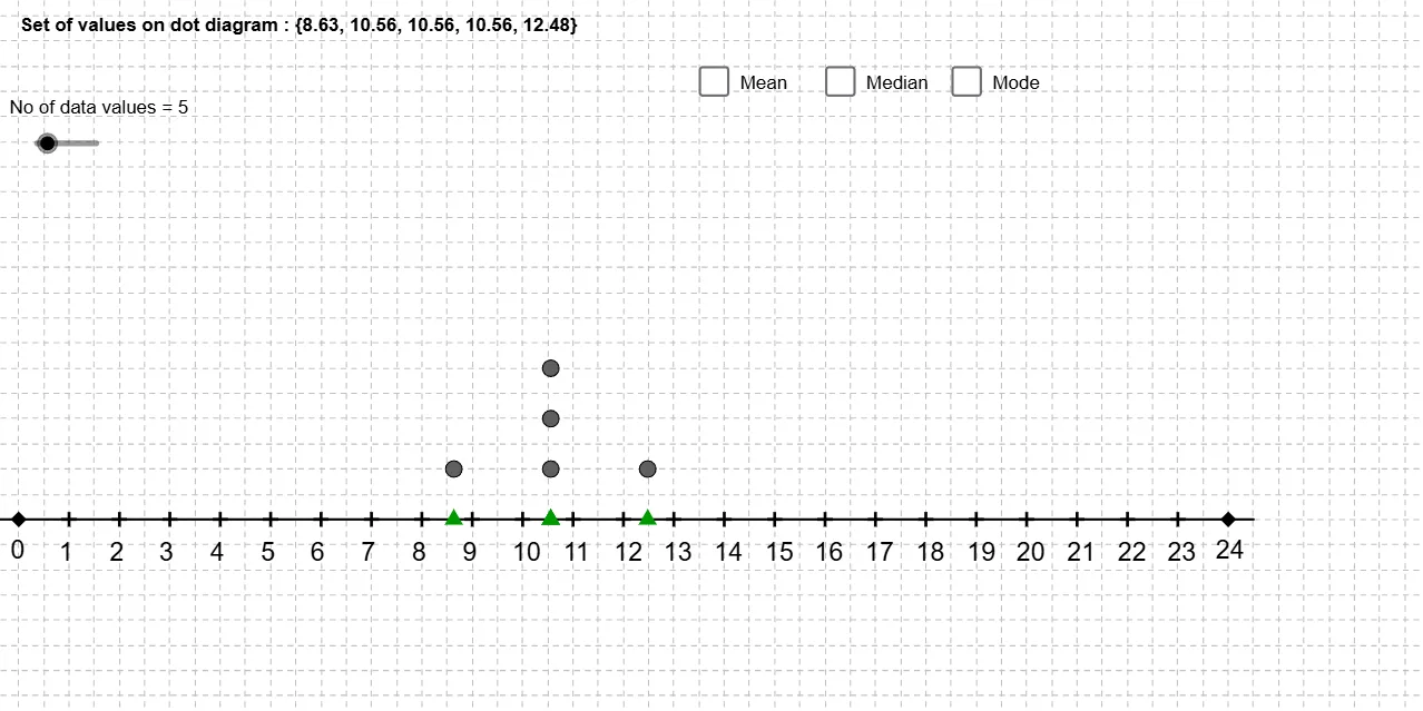
This example demonstrates how to change the data list of a dot plot by dragging points on the horizontal axis, with real-time visualization of mean and median calculations. Core math concepts include data distribution, mean (average), and median (middle value after sorting). Construction highlights the use of GeoGebra commands like Segment, Point, First, DotPlot, Sequence, and Join to create and dynamically update the dot plot and statistics. Suitable for middle school and above students in probability and statistics education to understand the representation of data central tendency.
GeoGebra Commands & Parameters
Segment((x(L_l) - 0.5, 0), (x(L_u) + 0.5, 0)) → aPoint(a) → APoint(a) → BPoint(a) → CPoint(a) → DPoint(a) → EPoint(a) → FPoint(a) → GPoint(a) → HPoint(a) → IPoint(a) → JPoint(a) → KPoint(a) → LSegment((0, (-v)), (0, v)) → lPoint(a) → MPoint(a) → NPoint(a) → OPoint(a) → PPoint(a) → QPoint(a) → RPoint(a) → SPoint(a) → TPoint(a) → UPoint(a) → VPoint(a) → WPoint(a) → ZFirst(list1, Items) → list2DotPlot(list2) → list3Segment((Median[list2], 0), (Median[list2], 4)) → d_1Segment((-3, (-v)), (-3, v)) → iSegment((8, (-v)), (8, v)) → a_1Segment((9, (-v)), (9, v)) → b_1Segment((-9, (-v)), (-9, v)) → cSegment((-8, (-v)), (-8, v)) → dSegment((-7, (-v)), (-7, v)) → eSegment((-6, (-v)), (-6, v)) → fSegment((-5, (-v)), (-5, v)) → gSegment((-4, (-v)), (-4, v)) → hSegment((-2, (-v)), (-2, v)) → jSegment((-1, (-v)), (-1, v)) → kSegment((1, (-v)), (1, v)) → mSegment((2, (-v)), (2, v)) → nSegment((3, (-v)), (3, v)) → pSegment((4, (-v)), (4, v)) → qSegment((6, (-v)), (6, v)) → sSegment((5, (-v)), (5, v)) → rSegment((7, (-v)), (7, v)) → tSegment((mean[list2], 0), (mean[list2], -3)) → e_1Segment((x(L_l), (-v)), (x(L_l), v)) → bSegment((x(L_u), (-v)), (x(L_u), v)) → c_1Sequence((p, 0), p, x(L_l) + 1, x(L_u) - 1, 1) → maintickSequence(Text[p, (p - 0.2, -0.8)], p, x(L_l) + 1, x(L_u) - 1, 1) → xaxislabelJoin({{Text[Element[list1, 1]]}, Sequence["+" + (Element[list1, i + 1]), i, 1, Items - 1]}) → listSum