
Integral Volume Y: Visualizing Volume of Revolution
Loading the math board and drawing, please wait…
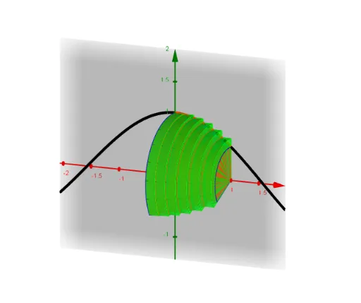
① This GeoGebra example dynamically demonstrates the computation of the volume of a solid of revolution obtained by rotating a function curve around the x-axis, using definite integrals and also showing left and right rectangle estimates. ② Core mathematical concepts include definite integrals, volume of revolution, Riemann sums, cylindrical shell method, and 3D visualization of surfaces and solids. ③ Construction highlights: commands such as Textfield, Integral, Sequence, Sum, Surface, and CircumcircleSector are used to create input boxes for limits, the definite integral area, left/right rectangle estimates, rotated cylinders, and curved surfaces, with sliders and input boxes for interactive parameter changes. ④ Suitable for high school to college calculus courses, helping students intuitively grasp the geometric meaning of integration for volume and numerical approximation methods.
GeoGebra Commands & Parameters
Textfield(f) → inputBox1Textfield(upperlimit) → inputBox2Textfield(lowerlimit) → inputBox3Integral(f, ll, ul) → AreabyDefiniteIntegralSequence(Polygon[(dx, 0), (dx, f(dx)), (dx + (ul - ll) / number, f(dx)), (dx + (ul - ll) / number, 0)], dx, ll, ul - (ul - ll) / number, (ul - ll) / number) → LeftRectanglesEstimateSum(LeftRectanglesEstimate) → AreaLeftRectangleEstimateSequence(Polygon[(dx, 0), (dx, f(dx + (ul - ll) / number)), (dx + (ul - ll) / number, f(dx + (ul - ll) / number)), (dx + (ul - ll) / number, 0)], dx, ll, ul - (ul - ll) / number, (ul - ll) / number) → RightRectanglesEstimateSum(RightRectanglesEstimate) → AreaRightRectangleEstimateSequence(x = dx, dx, ll, ul, (ul - ll) / number) → VerticalLinesWithinLimitsSequence((dx, f(dx)), dx, ll, ul, (ul - ll) / number) → PointsOnCurvefWithinLimitsSurface(fprime, θ, xAxis) → CurvedBoundaryCircumcircleSector((ll, f(ll), 0), (ll, (f(ll) * cos(θ / 3)), (f(ll) * sin(θ / 3))), (ll, (f(ll) * cos(θ)), (f(ll) * sin(θ)))) → LLDiscCircumcircleSector((ul, f(ul), 0), (ul, (f(ul) * cos(θ / 3)), (f(ul) * sin(θ / 3))), (ul, (f(ul) * cos(θ)), (f(ul) * sin(θ)))) → ULDiscSequence(Polygon[(dx, 0, 0), (dx, (f(dx) * cos(θ)), (f(dx) * sin(θ))), (dx + (ul - ll) / number, (f(dx) * cos(θ)), (f(dx) * sin(θ))), (dx + (ul - ll) / number, 0, 0)], dx, ll, ul - (ul - ll) / number, (ul - ll) / number) → LeftRectangleRotateSequence(CircumcircleSector[(dx, f(dx), 0), (dx, (f(dx) * cos(θ / 3)), (f(dx) * sin(θ / 3))), (dx, (f(dx) * cos(θ)), (f(dx) * sin(θ)))], dx, ll, ul - (ul - ll) / number, (ul - ll) / number) → LeftCylinderLeftSectorSequence(CircumcircleSector[(dx + (ul - ll) / number, f(dx), 0), (dx + (ul - ll) / number, (f(dx) * cos(θ / 3)), (f(dx) * sin(θ / 3))), (dx + (ul - ll) / number, (f(dx) * cos(θ)), (f(dx) * sin(θ)))], dx, ll, ul - (ul - ll) / number, (ul - ll) / number) → LeftCylinderRightSectorSequence(Surface[u, (f(dx) * cos(v)), (f(dx) * sin(v)), u, dx, dx + (ul - ll) / number, v, 0, θ], dx, ll, ul - (ul - ll) / number, (ul - ll) / number) → LeftCylinderCurvedSurfaceSequence(Cylinder[(dx, 0, 0), (dx + (ul - ll) / number, 0, 0), f(dx + (ul - ll) / number)], dx, ll, ul - (ul - ll) / number, (ul - ll) / number) → RightCylinderEstimateSequence(CircumcircleSector[(dx, f(dx + (ul - ll) / number), 0), (dx, (f(dx + (ul - ll) / number) * cos(θ / 3)), (f(dx + (ul - ll) / number) * sin(θ / 3))), (dx, (f(dx + (ul - ll) / number) * cos(θ)), (f(dx + (ul - ll) / number) * sin(θ)))], dx, ll, ul - (ul - ll) / number, (ul - ll) / number) → RightCylinderLeftSectorSequence(CircumcircleSector[(dx + (ul - ll) / number, f(dx + (ul - ll) / number), 0), (dx + (ul - ll) / number, (f(dx + (ul - ll) / number) * cos(θ / 3)), (f(dx + (ul - ll) / number) * sin(θ / 3))), (dx + (ul - ll) / number, (f(dx + (ul - ll) / number) * cos(θ)), (f(dx + (ul - ll) / number) * sin(θ)))], dx, ll, ul - (ul - ll) / number, (ul - ll) / number) → RightCylinderRightSectorSequence(Polygon[(dx, 0, 0), (dx, (f(dx + (ul - ll) / number) * cos(θ)), (f(dx + (ul - ll) / number) * sin(θ))), (dx + (ul - ll) / number, (f(dx + (ul - ll) / number) * cos(θ)), (f(dx + (ul - ll) / number) * sin(θ))), (dx + (ul - ll) / number, 0, 0)], dx, ll, ul - (ul - ll) / number, (ul - ll) / number) → RightRectangleRotateSum(RightCylinderEstimate) → VolumeRightCylinderEstimateSequence(Cylinder[(dx, 0, 0), (dx + (ul - ll) / number, 0, 0), f(dx)], dx, ll, ul - (ul - ll) / number, (ul - ll) / number) → LeftCylinderEstimateSum(LeftCylinderEstimate) → VolumeLeftCylinderEstimateIntegral(f(x)^(2)) → h_1Sequence(Surface[u, (f(dx + (ul - ll) / number) * cos(v)), (f(dx + (ul - ll) / number) * sin(v)), u, dx, dx + (ul - ll) / number, v, 0, θ], dx, ll, ul - (ul - ll) / number, (ul - ll) / number) → RightCylinderCurvedSurfaceSurface(u, (v * f(u)), 0, u, lowerlimit, upperlimit, v, 0, 1) → Areain3D
AI Drawing Prompt Reference
Visualize the volume of a solid of revolution formed by rotating a function curve around the x-axis using definite integrals, and include left and right rectangle estimates. The plot should feature input boxes for the function and integral limits, display the area of the definite integral, and show the left and right rectangle estimates. Include the rotated cylinders and curved surfaces, along with volume estimates for the left and right cylinders. Use sliders and input boxes for interactive parameter changes, presenting the rotation body, integral area, rectangle estimates, and 3D visualization of the solid.
The prompt above was compiled from the original drawing commands and is for reference only.