Rotating Solid Volume Around X and Y Axes

Loading the math board and drawing, please wait…

2018-05-06 10:31

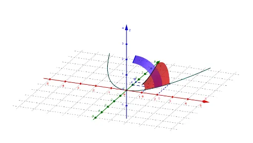
This example demonstrates how to generate a rotating solid by rotating a curve around the X-axis and Y-axis, and calculate its volume. The core mathematical concepts involved include the volume formula for rotating solids, parametric equations, logarithmic functions, and quadratic functions. Construction highlights extracted from the 'Construction Summary' using GeoGebra commands/objects: Textfield, Line, Intersect, CurveCartesian, Segment, Surface, Invert, Rotate, If; objects include d, f, c, rx, ry, φ, ϕ, Textfeld1, a, b, Textfeld2, Textfeld3, g_1, I, g_2, J, k, Textfeld4, Textfeld5, A, B, G, F, D, C, s_1, s_2, f_x, f_u, V_x, V_y, ff_u, Text1, Text2, s_3, s_4, k_x, k_y, f_y. Suitable for high school and above students to learn and understand the method of calculating the volume of rotating solids and the application of parametric equations.

GeoGebra Commands & Parameters

Textfield(f) → Textfeld1
Textfield(a) → Textfeld2
Textfield(b) → Textfeld3
Line((0, c), Vector[(1, 0)]) → g_1
Intersect(f, g_1, (1, f(1))) → I
Line((0, d), Vector[(1, 0)]) → g_2
Intersect(f, g_2, (d, f(d))) → J
CurveCartesian(t, f(t), 0, t, -5, 5) → k
Textfield(c) → Textfeld4
Textfield(d) → Textfeld5
Segment(A, G) → s_1
Segment(B, F) → s_2
Surface(u, (f(u) * cos(w)), (f(u) * sin(w)), u, a, b, w, 0, φ) → f_x
Invert(f) → f_u
Segment(C, I) → s_3
Segment(D, J) → s_4
Rotate(If[a ≤ x ≤ b, f], φ, xAxis) → k_x
If(f_u(c) < f_u(d), Rotate[If[f_u(c) ≤ x ≤ f_u(d), f(x)], (-ϕ), yAxis], Rotate[If[f_u(d) ≤ x ≤ f_u(c), f(x)], (-ϕ), yAxis]) → k_y
If(f_u(c) < f_u(d), Surface[(uu * cos(ww)), f(uu), (uu * sin(ww)), uu, f_u(c), f_u(d), ww, 0, ϕ], Surface[(uu * cos(ww)), f(uu), (uu * sin(ww)), uu, f_u(d), f_u(c), ww, 0, ϕ]) → f_y