Imagine: Ferriswheel—Circle Angles and Riemann-Sum Thinking

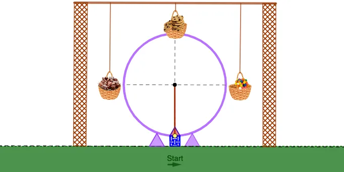
This GeoGebra example uses a Ferriswheel-inspired geometry scene to visualize how angle relationships change for points moving on a circle, and how those changing quantities can be organized into a partition-based summation viewpoint (upper/lower sum or Riemann-sum style) for approximating an accumulated value. The key math concepts include circle geometry and sectors (Circle, CircleSector), angle modeling (Angle), and symmetry via transformation (Mirror). It also highlights geometric reasoning with isosceles-triangle/angle constraints and supports an estimation framework connected to arithmetic mean through partitioned summations. Construction highlights: Circle defines the main orbit, Point together with Intersect and Segment establishes key locations and connections, OrthogonalLine provides perpendicular/projection structure, and Polygon assembles the ferriswheel-like outlines. Vector elements can encode direction from reference points to the moving positions, while Mirror replicates symmetric parts. The scene is built from many constructed objects (points, angles such as α, and polygons like poly1/poly2). Suitable for middle and high school geometry lessons on circles, angles, and constructions, and also for introductory calculus contexts where learners can intuit why partition sums (upper/lower sums or Riemann sums) approximate an integral or total effect.