
Hyperboloid as a Ruled Surface: Dynamic Construction
Loading the math board and drawing, please wait…
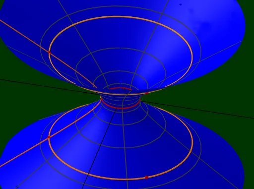
This GeoGebra example demonstrates how a one-sheeted hyperboloid is generated by a family of straight lines (rulings), visually illustrating its nature as a ruled surface. Core mathematical concepts include hyperboloids, ruled surfaces, parametric surfaces, spatial line families, and trigonometric parameterization. Construction highlights: the Surface command defines the hyperboloid's parametric equation, CurveCartesian creates spatial curves, and Line, Sequence, and Zip generate and arrange the ruling lines. A slider (e.g., α) dynamically adjusts the rulings, while auxiliary elements such as elliptical cross-sections, asymptotes, and projections are displayed. Suitable for high school to university levels in solid geometry, analytic geometry, or computer-assisted mathematics education, this example aids in understanding the generation mechanism and parametric representation of ruled surfaces.
GeoGebra Commands & Parameters
Surface(((a * cosh(u)) * cos(v)), ((b * cosh(u)) * sin(v)), (c * sinh(u)), u, -10, 10, v, (-π), π) → H_pCurveCartesian(H_p((-u), v), v, -10, 10) → ell_{-u}CurveCartesian(H_p(u, v), v, -10, 10) → ell_uCurveCartesian(H_p(0, v), v, (-π), π) → ell_0CurveCartesian((((a * cosh(u)) * cos(v)), ((b * cosh(u)) * sin(v)), (c * sinh(u))), u, -10, 10) → hyp_vLine((0, 0, 0), (1, 0, 0)) → g_xLine((0, 0, 0), (0, 1, 0)) → g_ySequence(k, k, 1, (m * n)) → l_nZip(Line[(((a * cosh(u)) * cos(v - α / 2 + (k / (m + 1) * α))), ((b * cosh(u)) * sin(v - α / 2 + (k / (m + 1) * α))), (c * sinh(u))), (((a * cosh((-u))) * cos(v + α / 2 + (k / (m + 1) * α))), ((b * cosh((-u))) * sin(v + α / 2 + (k / (m + 1) * α))), (c * sinh((-u))))], k, l_n) → ListErz_nZip(Line[(((a * cosh(u)) * cos(v + α / 2 - (k / (m + 1) * α))), ((b * cosh(u)) * sin(v + α / 2 - (k / (m + 1) * α))), (c * sinh(u))), (((a * cosh((-u))) * cos(v - α / 2 - (k / (m + 1) * α))), ((b * cosh((-u))) * sin(v - α / 2 - (k / (m + 1) * α))), (c * sinh((-u))))], k, l_n) → ListErz'_nSurface(((a * cosh(u)) * ((λ * cos(v + α)) + ((1 - λ) * cos(v)))), ((b * cosh(u)) * ((λ * sin(v + α)) + ((1 - λ) * sin(v)))), ((c * sinh(u)) * ((2 * λ) - 1)), v, (-π), π, λ, -10, 10) → H'_{erz}Surface(((a * cosh(u)) * ((λ * cos(v)) + ((1 - λ) * cos(v + α)))), ((b * cosh(u)) * ((λ * sin(v)) + ((1 - λ) * sin(v + α)))), ((c * sinh(u)) * ((2 * λ) - 1)), v, (-π), π, λ, -10, 10) → H_{erz}CurveCartesian((a * (((λ * cosh(u)) * cos(v)) + (((1 - λ) * cosh((-u))) * cos(v + α)))), (b * (((λ * cosh(u)) * sin(v)) + (((1 - λ) * cosh((-u))) * sin(v + α)))), (c * ((λ * sinh(u)) + ((1 - λ) * sinh((-u))))), λ, -10, 10) → erzeugende_{+}CurveCartesian((a * (((λ * cosh(u)) * cos(v + α)) + (((1 - λ) * cosh((-u))) * cos(v)))), (b * (((λ * cosh(u)) * sin(v + α)) + (((1 - λ) * cosh((-u))) * sin(v)))), (c * ((λ * sinh(u)) + ((1 - λ) * sinh((-u))))), λ, -10, 10) → erzeugende_{-}CurveCartesian(((1 / 2 * cosh(u)) * ((a * (cos(v) + cos(v + α))), (b * (sin(v) + sin(v + α))), 0)), v, (-π), π) → sPkt
AI Drawing Prompt Reference
Draw a one-sheeted hyperboloid to illustrate that it is generated by a family of straight lines, showcasing it as a ruled surface. Start by plotting the parametric surface equation of the hyperboloid, then create the ruling lines which are spatial curves. Dynamically adjust a parameter α to show the movement of these lines. Also display elliptical cross-sections, asymptotes, and projections to aid in understanding the generation mechanism and parametric representation.
The prompt above was compiled from the original drawing commands and is for reference only.