
Horizontal Compression of Sine and Cosine Functions
Loading the math board and drawing, please wait…
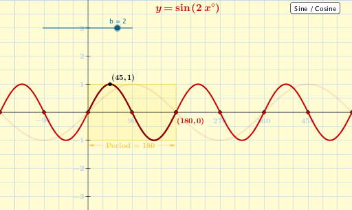
①This GeoGebra example dynamically demonstrates the horizontal compression of the sine function y=sin(x) and cosine function y=cos(x), showing how the graph changes when the period (frequency) is altered. ②The core mathematical concept is the horizontal scaling of trigonometric functions (y=f(kx)), relating to period and frequency transformations. ③Construction highlights: uses CurveCartesian to plot the sine and cosine curves, a slider to control the compression factor, and various objects such as Sequence, Polygon, Vector, and multiple text labels (text1 to text17) to display expressions and parameters. ④Suitable for high school or introductory college students learning trigonometric transformations, and useful for classroom demonstrations or self-study to visualize the effect of parameter changes on function graphs.
GeoGebra Commands & Parameters
Corner(5) → BSequence(Segment[((90 * n), (-dd)), ((90 * n), dd)], n, -2, 6) → list1Sequence(((90 * n), 0), n, -2, 6) → list3Sequence((0, n), n, -3, 3) → list5Sequence(Segment[((-57.3 * dd), n), ((57.3 * dd), n)], n, -3, 3) → list2Sequence(((180 * n / b), 0), n, -9, 9) → list4Sequence(((90 + (180 * n)) / b, 0), n, -9, 9) → list6Polygon((0, (-a)), (360 / b, (-a)), (360 / b, a), (0, a)) → poly1, i, j, k, lVector(((x(Corner[text21, 1]) + x(Corner[text21, 4])) / 2, (y(Corner[text21, 1]) + y(Corner[text21, 4])) / 2), (Min[0, 360 / b], (y(Corner[text21, 1]) + y(Corner[text21, 4])) / 2)) → uVector(((x(Corner[text21, 2]) + x(Corner[text21, 3])) / 2, (y(Corner[text21, 1]) + y(Corner[text21, 4])) / 2), (Max[0, 360 / b], (y(Corner[text21, 1]) + y(Corner[text21, 4])) / 2)) → vCurveCartesian(t, (a * cos(((b * t))°)), t, Min[0, 360 / b], Max[0, 360 / b]) → dCurveCartesian(t, (a * sin(((b * t))°)), t, Min[0, 360 / b], Max[0, 360 / b]) → c
AI Drawing Prompt Reference
Draw a coordinate system showing horizontal compression of sine and cosine functions. The x-axis is in degrees, y-axis is function values. Use a slider to control the compression factor, making the sine and cosine curves stretch or shrink horizontally, changing their periods. Include a rectangle highlighting one full period, with arrows at its edges indicating compression direction. Mark key angles (multiples of 90 and 180 degrees) on the x-axis, and draw grid lines both vertically and horizontally. Add text labels displaying the function expressions, current parameter values, and notes about period changes, to visually demonstrate how horizontal scaling affects the graphs.
The prompt above was compiled from the original drawing commands and is for reference only.