
Half-Life Dynamic Geometric Illustration
Loading the math board and drawing, please wait…
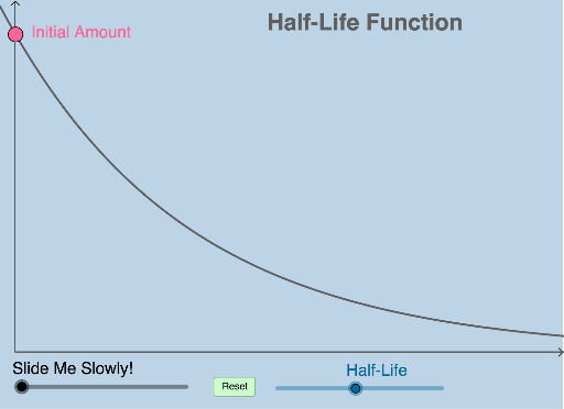
This GeoGebra example dynamically visualizes the half-life of a radioactive element, illustrating exponential decay through interactive geometric transformations. Users adjust initial quantity and decay coefficient via input boxes or sliders, observing real-time changes in the decay curve and associated geometric figures. Core mathematical concepts include exponential functions, half-life formulas, and the correspondence between geometric dilations and proportional decay rates. Construction leverages GeoGebra commands such as Textfield for parameter input, Dilate, Rotate, Translate, Vector, Ray, and Integral for computing accumulated decay or area under the curve, alongside Intersect, Segment, and Midpoint for precise point and segment management. The model is suitable for high school exponential function units, calculus applications of integrals in accumulation contexts, or physics-based radioactive decay modeling, serving both teacher-led demonstrations and student-driven inquiry.
GeoGebra Commands & Parameters
Textfield(a_0) → InputBox1Textfield(k) → InputBox2Intersect(A, b, (475.00000000000006, 608.7077589414912)) → DIntersect(A, c, (950, 304.35387947074565)) → EIntersect(A, d, (1425, 152.17693973537283)) → FIntersect(A, e, (1900, 76.08846986768641)) → GTextfield(f) → InputBox3Intersect(b, h) → HSegment(H, D) → iIntersect(c, j) → IIntersect(d, l) → JSegment(I, E) → mSegment(J, F) → nSegment(D, I) → pSegment(E, J) → qIntersect(h, s) → KIntersect(r, t) → LSegment(K, C) → f_1Segment(C, L) → g_1Midpoint(M, B) → NDilate(M, If[0 < o ≤ 1, 1 - o, 0], N) → M'Rotate(M, If[1 < o ≤ 2, ((o - 1) * π), π], N) → M'_1Rotate(M', If[1 < o ≤ 2, ((o - 1) * π), π], N) → M''Dilate(N, If[2 < o ≤ 3, 3 - o, 0], D) → N'Segment(N, N') → j_1Midpoint(D, O) → RDilate(B, If[0 < o ≤ 1, 1 - o, 0], N) → B'Segment(B, B') → h_1Rotate(B, If[1 < o ≤ 2, ((-(o - 1)) * π), (-π)], N) → B'_1Rotate(B', If[1 < o ≤ 2, ((-(o - 1)) * π), (-π)], N) → B''Segment(B'_1, B'') → i_1Dilate(D, If[3 < o ≤ 4, 4 - o, 0], R) → D'Segment(D, D') → k_1Dilate(R, If[4 < o ≤ 5, 5 - o, 0], O) → R'Segment(R, R') → l_1Rotate(D, If[5 < o ≤ 6, ((-(o - 5)) * π), (-π)], R) → D'_1Rotate(D', If[5 < o ≤ 6, ((-(o - 5)) * π), (-π)], R) → D''Segment(D'_1, D'') → m_1Rotate(N, If[6 < o ≤ 7, ((-(o - 6)) * π), (-π)], D) → N'_1Rotate(N', If[6 < o ≤ 7, ((-(o - 6)) * π), (-π)], D) → N''Segment(N'_1, N'') → n_1Dilate(D, If[7 < o ≤ 8, 8 - o, 0], R) → D'_2Vector(D, D'_2) → uTranslate(N'_1, u) → STranslate(N'', u) → N'''Segment(S, N''') → p_1Midpoint(P, E) → TDilate(E, If[8 < o ≤ 9, 9 - o, 0], T) → E'Segment(E, E') → q_1Dilate(T, If[9 < o ≤ 10, 10 - o, 0], P) → T'Segment(T, T') → r_1Rotate(E, If[10 < o ≤ 11, ((-(o - 10)) * π), (-π)], T) → E'_1Rotate(E', If[10 < o ≤ 11, ((-(o - 10)) * π), (-π)], T) → E''Segment(E'_1, E'') → s_1Rotate(S, If[11 < o ≤ 12, ((-(o - 11)) * π), (-π)], E) → S'Rotate(N''', If[11 < o ≤ 12, ((-(o - 11)) * π), (-π)], E) → USegment(S', U) → t_1Dilate(E, If[12 < o ≤ 13, 13 - o, 0], T) → E'_2Vector(E, E'_2) → vTranslate(S', v) → S''Translate(U, v) → U'Segment(S'', U') → a_1Midpoint(F, Q) → VDilate(F, If[13 < o ≤ 14, 14 - o, 0], V) → F'Segment(F, F') → b_1Dilate(V, If[14 < o ≤ 15, 15 - o, 0], Q) → V'Segment(V, V') → c_1Rotate(F, If[15 < o ≤ 16, ((-(o - 15)) * π), (-π)], V) → F'_1Rotate(F', If[15 < o ≤ 16, ((-(o - 15)) * π), (-π)], V) → F''Segment(F'_1, F'') → d_1Rotate(S'', If[16 < o ≤ 17, ((-(o - 16)) * π), (-π)], F) → S'''Rotate(U', If[16 < o ≤ 17, ((-(o - 16)) * π), (-π)], F) → U''Segment(S''', U'') → e_1Dilate(F, If[17 < o ≤ 18, 18 - o, 0], V) → F'_2Vector(F, F'_2) → wTranslate(S''', w) → WTranslate(U'', w) → U'''Segment(W, U''') → f_2Translate(U'', w) → U'''_1Ray((0, 0), (1, 0)) → g_2Integral(A, 0, (50 * k)) → o_1