
Half-Life Dynamic Demonstration
Loading the math board and drawing, please wait…
In collections
Exploring Exponential & Logarithmic Functions
Exploring Exponential & Logarithmic Functions
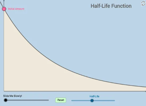
This example demonstrates the dynamic process of an element's half-life, involving exponential functions. By adjusting parameters, observe the changes in half-life. It uses GeoGebra commands such as Textfield, Intersect, Segment, etc., suitable for high school and above students to learn about exponential functions and their applications.
GeoGebra Commands & Parameters
Textfield(a_0) → InputBox1Textfield(k) → InputBox2Intersect(A, b, (475.00000000000006, 608.7077589414912)) → DIntersect(A, c, (950, 304.35387947074565)) → EIntersect(A, d, (1425, 152.17693973537283)) → FIntersect(A, e, (1900, 76.08846986768641)) → GTextfield(f) → InputBox3Intersect(b, h) → HSegment(H, D) → iIntersect(c, j) → IIntersect(d, l) → JSegment(I, E) → mSegment(J, F) → nSegment(D, I) → pSegment(E, J) → qIntersect(h, s) → KIntersect(r, t) → LSegment(K, C) → f_1Segment(C, L) → g_1Midpoint(M, B) → NDilate(M, If[0 < o ≤ 1, 1 - o, 0], N) → M'Rotate(M, If[1 < o ≤ 2, ((o - 1) * π), π], N) → M'_1Rotate(M', If[1 < o ≤ 2, ((o - 1) * π), π], N) → M''Dilate(N, If[2 < o ≤ 3, 3 - o, 0], D) → N'Segment(N, N') → j_1Midpoint(D, O) → RDilate(B, If[0 < o ≤ 1, 1 - o, 0], N) → B'Segment(B, B') → h_1Rotate(B, If[1 < o ≤ 2, ((-(o - 1)) * π), (-π)], N) → B'_1Rotate(B', If[1 < o ≤ 2, ((-(o - 1)) * π), (-π)], N) → B''Segment(B'_1, B'') → i_1Dilate(D, If[3 < o ≤ 4, 4 - o, 0], R) → D'Segment(D, D') → k_1Dilate(R, If[4 < o ≤ 5, 5 - o, 0], O) → R'Segment(R, R') → l_1Rotate(D, If[5 < o ≤ 6, ((-(o - 5)) * π), (-π)], R) → D'_1Rotate(D', If[5 < o ≤ 6, ((-(o - 5)) * π), (-π)], R) → D''Segment(D'_1, D'') → m_1Rotate(N, If[6 < o ≤ 7, ((-(o - 6)) * π), (-π)], D) → N'_1Rotate(N', If[6 < o ≤ 7, ((-(o - 6)) * π), (-π)], D) → N''Segment(N'_1, N'') → n_1Dilate(D, If[7 < o ≤ 8, 8 - o, 0], R) → D'_2Vector(D, D'_2) → uTranslate(N'_1, u) → STranslate(N'', u) → N'''Segment(S, N''') → p_1Midpoint(P, E) → TDilate(E, If[8 < o ≤ 9, 9 - o, 0], T) → E'Segment(E, E') → q_1Dilate(T, If[9 < o ≤ 10, 10 - o, 0], P) → T'Segment(T, T') → r_1Rotate(E, If[10 < o ≤ 11, ((-(o - 10)) * π), (-π)], T) → E'_1Rotate(E', If[10 < o ≤ 11, ((-(o - 10)) * π), (-π)], T) → E''Segment(E'_1, E'') → s_1Rotate(S, If[11 < o ≤ 12, ((-(o - 11)) * π), (-π)], E) → S'Rotate(N''', If[11 < o ≤ 12, ((-(o - 11)) * π), (-π)], E) → USegment(S', U) → t_1Dilate(E, If[12 < o ≤ 13, 13 - o, 0], T) → E'_2Vector(E, E'_2) → vTranslate(S', v) → S''Translate(U, v) → U'Segment(S'', U') → a_1Midpoint(F, Q) → VDilate(F, If[13 < o ≤ 14, 14 - o, 0], V) → F'Segment(F, F') → b_1Dilate(V, If[14 < o ≤ 15, 15 - o, 0], Q) → V'Segment(V, V') → c_1Rotate(F, If[15 < o ≤ 16, ((-(o - 15)) * π), (-π)], V) → F'_1Rotate(F', If[15 < o ≤ 16, ((-(o - 15)) * π), (-π)], V) → F''Segment(F'_1, F'') → d_1Rotate(S'', If[16 < o ≤ 17, ((-(o - 16)) * π), (-π)], F) → S'''Rotate(U', If[16 < o ≤ 17, ((-(o - 16)) * π), (-π)], F) → U''Segment(S''', U'') → e_1Dilate(F, If[17 < o ≤ 18, 18 - o, 0], V) → F'_2Vector(F, F'_2) → wTranslate(S''', w) → WTranslate(U'', w) → U'''Segment(W, U''') → f_2Translate(U'', w) → U'''_1Ray((0, 0), (1, 0)) → g_2Integral(A, 0, (50 * k)) → o_1
AI Drawing Prompt Reference
Create a diagram illustrating the dynamic process of an element's half-life. Include an exponential decay curve, with several equally spaced vertical lines intersecting the curve at points that drop down to the horizontal axis, forming a series of decreasing-height bars. Add adjustable input fields or sliders below the curve to control the initial amount and decay constant. Also incorporate auxiliary line segments and animated rotation/scaling effects to simulate particle movement during nuclear decay, with a clear layout for observing half-life changes.
The prompt above was compiled from the original drawing commands and is for reference only.