
Logarithmic Action (3)! – Dynamic Discovery of the Power Property
Loading the math board and drawing, please wait…
In collections
Exploring Exponential & Logarithmic Functions
Exploring Exponential & Logarithmic Functions
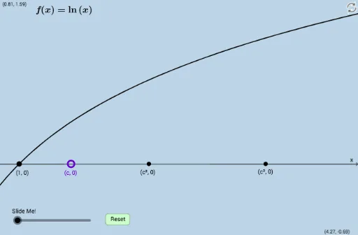
① This interactive GeoGebra construction visually demonstrates the power property of logarithms (log_b(a^n) = n·log_b(a)) through a dynamic, modifiable discovery environment. ② Core mathematical concepts include logarithmic functions, the power rule for logarithms, function transformations, and coordinate geometry involving points, segments, vectors, and distances. ③ The construction employs GeoGebra commands such as Textfield, InputBox, Intersect, Dilate, Segment, Vector, Translate, Rotate, Distance, Midpoint, Line, and Circle to create a rich set of objects (points A, B, C, D, E, F and their primed variants) that respond to user input, allowing real-time comparison of the two sides of the logarithmic identity. ④ This resource is ideal for high school students learning logarithmic properties, as well as for teachers seeking an interactive demonstration to foster conceptual understanding and inquiry-based exploration.
GeoGebra Commands & Parameters
Textfield(a) → InputBox1Textfield(f_1) → InputBox2Textfield(f) → InputBox3Intersect(f, h, 1) → EDilate(F, If[0 < d ≤ 1, 1 - d, 0], A) → F'Dilate(A, If[1 < d ≤ 2, 2 - d, 0], B) → A'Segment(A, A') → jDilate(B, If[2 < d ≤ 3, 3 - d, 0], G) → B'Vector(B, B') → uTranslate(A, u) → A'_1Translate(A', u) → A''Segment(A'_1, A'') → j'Rotate(A'_1, If[3 < d ≤ 4, ((-(d - 3)) * π / 2), ((-π)) / 2], F) → HRotate(A'', If[3 < d ≤ 4, ((-(d - 3)) * π / 2), ((-π)) / 2], F) → A'''Segment(H, A''') → j''Rotate(A'_1, If[3 < d ≤ 4, ((d - 3) * π / 2), π / 2], F) → IRotate(A'', If[3 < d ≤ 4, ((d - 3) * π / 2), π / 2], F) → A'''_1Dilate(D, If[4 < d ≤ 5, 5 - d, 0], E) → D'Segment(D, D') → lDilate(A, If[1 < d ≤ 2, 2 - d, 0], C) → A'_2Segment(A, A'_2) → mDilate(A, If[2 < d ≤ 3, 3 - d, 0], R) → C'Vector(C, C') → vIntersect(f, p, 1) → NRotate(F, If[5 < d ≤ 6, ((d - 5) * π / 2), π / 2], F) → F'_1Rotate(F', If[5 < d ≤ 6, ((d - 5) * π / 2), π / 2], F) → F''Dilate(F, If[6 < d ≤ 7, 7 - d, 0], M) → F'_2Vector(F, F'_2) → wTranslate(F'_1, w) → PTranslate(F'', w) → F'''Distance(A, C) → distanceACVector(A, A'_2) → iVector(A, C') → b_1Midpoint(Z, A_1) → QLine(B_1, C_1) → eSegment(B_1, C_1) → g_1Circle(B_1, g_1 / 3) → c_1Intersect(c_1, e, 2) → TCircle(T, g_1 / 3) → d_1Intersect(d_1, e, 2) → UDilate(Z, If[2 < d ≤ 3, 3 - d, 0], Q) → Z'Segment(Z, Z') → qDilate(Q, If[3 < d ≤ 4, 4 - d, 0], A_1) → Q'Segment(Q, Q') → h_1Dilate(B_1, If[4 < d ≤ 5, 5 - d, 0], T) → D_1Segment(B_1, D_1) → i_1Dilate(T, If[5 < d ≤ 6, 6 - d, 0], U) → T'Segment(T, T') → j_1Dilate(U, If[6 < d ≤ 7, 7 - d, 0], C_1) → U'Segment(U, U') → k_1Segment(A, A'_2) → l_1Distance(Z, A_1) → distanceZA1Distance(B_1, C_1) → distanceB1C1Dilate(A, If[7 < d ≤ 8, 8 - d, 0], Z) → A'_3Vector(A, A'_3) → u_1Dilate(A, If[7 < d ≤ 8, 8 - d, 0], B_1) → A'_4Vector(A, A'_4) → v_1Translate(A, u_1) → A'_5Translate(A'_2, u_1) → LSegment(A'_5, L) → m_1Translate(A, v_1) → A'_6Translate(A'_2, v_1) → WSegment(A'_6, W) → n_1Rotate(A'_5, If[8 < d ≤ 9, ((d - 8) * π), π], Q) → E_1Rotate(L, If[8 < d ≤ 9, ((d - 8) * π), π], Q) → L'Segment(E_1, L') → p_1Rotate(A'_6, If[8 < d ≤ 9, ((d - 8) * π), π], T) → F_1Rotate(W, If[8 < d ≤ 9, ((d - 8) * π), π], T) → W'Segment(F_1, W') → q_1Rotate(F_1, If[9 < d ≤ 10, ((d - 9) * π), π], U) → G_1Rotate(W', If[9 < d ≤ 10, ((d - 9) * π), π], U) → W''Segment(G_1, W'') → r_1
AI Drawing Prompt Reference
Create a dynamic illustration showing the power property of logarithms with two adjustable inputs and a logarithmic function graph. Display two geometric constructions involving scaled and rotated points, segments, and vectors that correspond to both sides of the logarithmic identity. The illustration should update in real-time as inputs change, clearly showing the relationship between the two constructions to visually prove the power rule for logarithms.
The prompt above was compiled from the original drawing commands and is for reference only.