Graphs and Correspondence Rules-2

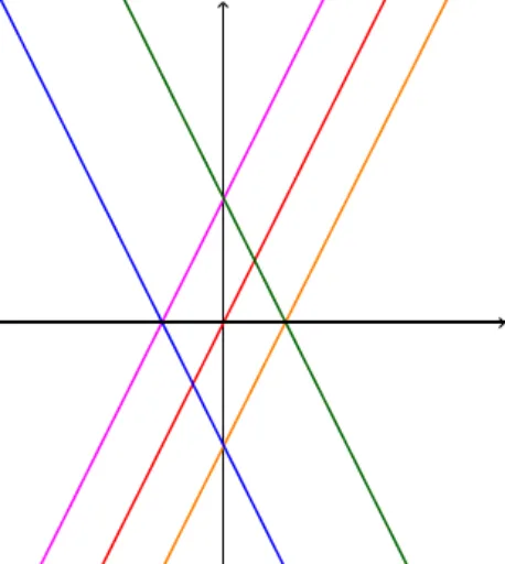
This example demonstrates the correspondence rules between 3D solids and 2D graphs through rotation, transformation, and linear equations. Core math concepts include rotation, solid geometry, linear equations, statistical characteristics, and diagrams. GeoGebra commands like LaTeX, TableText, and Textfield, along with objects such as f_1 to f_18, p_1 to p_6, InputBoxes 5 to 9, and variables a to e, are used to construct function graphs, text inputs, and parameter controls. Suitable for high school students learning solid geometry, coordinate geometry, and function graphing to understand spatial transformations and correspondence rules.