
Graphing the Absolute Value of a Quadratic Function
Loading the math board and drawing, please wait…
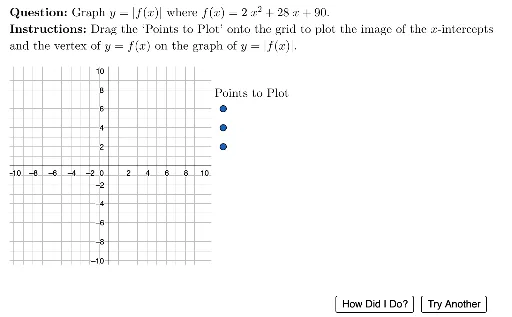
This example demonstrates how to graph the absolute value of a quadratic function. Key mathematical concepts include quadratic functions and absolute value functions. Using GeoGebra commands such as Flatten, Sequence, and Point, you can dynamically adjust parameters and observe changes in the graph. Suitable for high school mathematics education and learning about quadratic function graph transformations.
GeoGebra Commands & Parameters
Flatten(Sequence[Sequence[(i, j), i, -10, 10], j, 0, 10]) → GridSpaceSequence((12, i), i, 2, 6, 2) → homeSpacePoint(Union[GridSpace, {Element[homeSpace, 1]}]) → P_1Point(Union[GridSpace, {Element[homeSpace, 2]}]) → P_2Point(Union[GridSpace, {Element[homeSpace, 3]}]) → P_3Random(-10, 4) → Root1Random(1, floor(maxAval)) → aValExpand(((aVal * (x - Root1)) * (x - Root2))) → fUnicodeToLetter(10007) → xmarkUnicodeToLetter(10003) → cmarkPolygon({bottomLeft, (x(bottomLeft), y(topRight)), topRight, (x(topRight), y(bottomLeft))}) → viewboxPoint(Union[GridSpace, homeSpace]) → ActivePointLaTeX(ActivePoint) → activePtLblLaTeX(Expand[f]) → LblfLaTeX((("\text{Consider \(y=" * Lblf) * "\). Factoring, we get:}")) → fbLine2LaTeX((("\text{\(" * Factor[f]) * "\)}")) → fbLine4LaTeX(((("\text{\(" * Lblf) * "=") * If[aVal ≠ 1, (((((("" * aVal) * "(") * Expand[((x - Root1) * (x - Root2))]) * ")\)\\\phantom{") * Lblf) * "}="), "\)}"])) → fbLine3LaTeX((("\text{From this factored form, we conclude that the \\graph of \(y=" * f) * "\):}")) → fbLine5UnicodeToLetter(8226) → bulletLaTeX((((((("\text{\hphantom{12}" * bullet) * " has zeros \(") * Root1) * "\) and \(") * Root2) * "\),\\}")) → fbLine6LaTeX((((("\text{\hphantom{12}" * bullet) * " has axis of symmetry \(x =") * xCoordVertex) * "\), and}")) → fbLine7LaTeX((("(" * xCoordVertex) * ")")) → subStrIndexOf("x", Lblf) → firstXIf(Defined[firstX], IndexOf["x", Take[Lblf, firstX + 1]] + firstX) → secondXLaTeX(If[Defined[firstX], (Take[Lblf, 1, firstX - 1] * subStr), ""]) → subFirstXLaTeX((subFirstX * If[Defined[secondX], (Take[Lblf, firstX + 1, secondX - 1] * subStr), Take[Lblf, firstX + 1]])) → subSecondXLaTeX((subSecondX * If[Defined[secondX] ∧ secondX < Length[Lblf], Take[Lblf, secondX + 1], ""])) → subCompleteLaTeX("") → fbLine1LaTeX((((((("\text{\hphantom{12}" * bullet) * " \(y_\text{vertex}=") * subComplete) * "=") * yCoordVertex) * "\) is the \\ \(y\)-coordinate of the vertex.}")) → fbLine8Sequence((("SetFixed(P_" * i) * ",false,false)"), i, 1, 3) → testLaTeX((((((((("\text{Therefore, the vertex is \((" * xCoordVertex) * ",") * yCoordVertex) * ")\), which maps to\\\((") * xCoordVertex) * ",") * abs(yCoordVertex)) * ")\) on \(y= \left\vert f(x) \right\vert\) .}")) → fbLine9LaTeX((((((((((((((((fbLine1 * "\\") * fbLine2) * "\\") * fbLine3) * fbLine4) * "\\") * fbLine5) * "\\") * fbLine6) * "\\") * fbLine7) * "\\") * fbLine8) * "\\") * fbLine9)) → fbCompleteLaTeX((((("\text{\textbf{Question: }" * MainInstruc) * "\\\textbf{Instructions: }") * SpecInstruc) * "}")) → allInstruc
AI Drawing Prompt Reference
Draw the absolute value of a quadratic function. First, create a grid, then place three points on the grid representing the roots and vertex of the quadratic function. Randomly generate an a value and one root, then calculate the other root. Use these roots to construct the quadratic function and display its expanded form. Next, find the coordinates of the vertex and determine its corresponding point on the absolute value function graph.
The prompt above was compiled from the original drawing commands and is for reference only.