
Graphing a Polynomial with Complex Coefficients in the Complex Plane
Loading the math board and drawing, please wait…
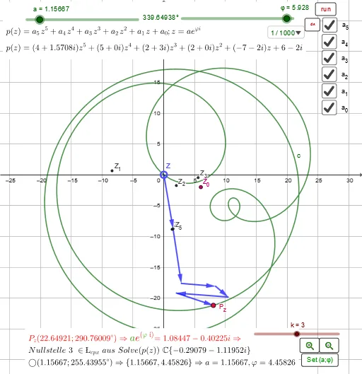
This example demonstrates how to visualize a complex-coefficient polynomial on the Gauss (complex) coordinate plane, linking the algebraic structure to geometric behavior. It highlights key ideas such as complex numbers, complex polynomials, and the geometric meaning behind the Fundamental Theorem of Algebra (existence of complex roots), together with tangent-related intuition and intersections that can be inferred from constructed curves. The construction starts by creating important points related to roots/coefficients (e.g., V_0…V_6 and Z_0…Z_5, Z) and then building the main graphical objects via GeoGebra’s core tools: CurveCartesian to draw the polynomial-related Cartesian curve, Translate to position/align components, Point to place the critical complex-plane points, Sequence to generate ordered collections of points, and Circle as auxiliary geometry. The resulting figure provides an interactive way to explore how varying parameters (slider-like objects such as k and angles/phase parameters) affects the plotted structure. Suitable for advanced high school and early undergraduate students studying complex numbers, algebra, and graphing/visualization in mathematics education.
GeoGebra Commands & Parameters
CurveCartesian((V_5 * ((a^(5) * pr(a_5)); (5 * t) + pi(a_5))) + (V_4 * ((a^(4) * pr(a_4)); (4 * t) + pi(a_4))) + (V_3 * ((a^(3) * pr(a_3)); (3 * t) + pi(a_3))) + (V_2 * ((a^(2) * pr(a_2)); (2 * t) + pi(a_2))) + (V_1 * ((a * pr(a_1)); t + pi(a_1))) + (V_0 * (pr(a_0); pi(a_0))), t, 0, (2 * π)) → cTranslate(Vector[(V_5 * Vector[Z_5])], (0, 0)) → v_1Translate(Vector[(V_4 * Vector[Z_4])], (V_5 * Z_5)) → v_2Translate(Vector[(V_3 * Vector[Z_3])], (V_5 * Z_5) + (V_4 * Z_4)) → v_3Translate(Vector[(V_2 * Vector[Z_2])], (V_5 * Z_5) + (V_4 * Z_4) + (V_3 * Z_3)) → v_4Translate(Vector[(V_1 * Vector[Z_1])], (V_5 * Z_5) + (V_4 * Z_4) + (V_3 * Z_3) + (V_2 * Z_2)) → v_5Translate(Vector[(V_0 * Vector[Z_0])], (V_5 * Z_5) + (V_4 * Z_4) + (V_3 * Z_3) + (V_2 * Z_2) + (V_1 * Z_1)) → v_6Point(Element[L_{cpx} + (0 * ί), k]) → LiSequence(Flatten[{xpol(Element[L_{cpx}, j]), ypol(Element[L_{cpx}, j])}], j, 1, Length[L_{cpx}]) → L_{pol}Circle(Element[{(V_0 * Z_0), (V_1 * Z_1), (V_2 * Z_2), (V_3 * Z_3), (V_4 * Z_4), (V_5 * Z_5)}, Max[{(V_5 * 6), (V_4 * 5), (V_3 * 4), (V_2 * 3), (V_1 * 2)}]], Sum[d] - Element[d, Max[{(V_5 * 6), (V_4 * 5), (V_3 * 4), (V_2 * 3), (V_1 * 2)}]]) → q
AI Drawing Prompt Reference
Draw a complex-plane graph that visualizes a polynomial with complex coefficients. First construct the main Cartesian curve determined by six complex-coefficient terms, incorporating amplitude-like weights from V0…V5 and phase shifts from the corresponding angles (a0…a5) and their real/imaginary parts. Then place a sequence of key points on the complex plane, using the constructed direction/offset elements Z0…Z5 (scaled by V0…V5) and positioned by successive translations so the point chain aligns with the structure used in the curve. Include the derived ordered coordinate sequence obtained from the polynomial mapping of those complex points (its real and imaginary coordinate components as x and y). Finally add an auxiliary circle whose center is based on the same V·Z combinations from the key points and whose radius is set by a maximum index constraint involving V1…V5, to help infer intersections and tangency intuition.
The prompt above was compiled from the original drawing commands and is for reference only.