
Visualizing Complex Roots of Quadratic Equations
Loading the math board and drawing, please wait…
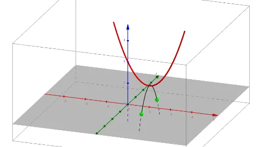
This GeoGebra example dynamically visualizes the complex roots of quadratic equations by representing them as geometric figures in the complex plane. It demonstrates how roots that are not real still have meaningful geometric counterparts, often appearing as intersections or loci related to conic sections such as hyperbolas. Core mathematical concepts include quadratic equations, complex numbers, discriminants, conic sections, and the relationship between coefficients and roots. The construction uses GeoGebra commands such as If, Sequence, and Conic, along with objects like lists (list1 to list5), points (A, B), and sliders (a, b, c) to adjust coefficients in real time)Skip. Suitable for high school and undergraduate students, this interactive tool bridges algebraic solving and geometric visualization, making abstract complex roots tangible and intuitive.
GeoGebra Commands & Parameters
If(b^(2) - ((4 * a) * c) ≥ 0, ((-b) + sqrt(b^(2) - ((4 * a) * c))) / ((2 * a)), ((-b)) / ((2 * a))) → s_{1a}If(b^(2) - ((4 * a) * c) ≥ 0, ((-b) - sqrt(b^(2) - ((4 * a) * c))) / ((2 * a)), ((-b)) / ((2 * a))) → s_{2a}If(b^(2) - ((4 * a) * c) ≥ 0, 0, sqrt(((4 * a) * c) - b^(2)) / ((2 * a))) → s_{1b}If(b^(2) - ((4 * a) * c) ≥ 0, 0, ((-sqrt(((4 * a) * c) - b^(2)))) / ((2 * a))) → s_{2b}Sequence((Element[list1, i], 0, Element[list2, i]), i, 1, 5) → list3Conic(Element[list3, 1], Element[list3, 2], Element[list3, 3], Element[list3, 4], Element[list3, 5]) → dSequence((v, Element[list1, i], Element[list4, i]), i, 1, 5) → list5Conic(Element[list5, 1], Element[list5, 2], Element[list5, 3], Element[list5, 4], Element[list5, 5]) → e
AI Drawing Prompt Reference
Visualize the complex roots of quadratic equations in the complex plane by dynamically adjusting coefficients a, b, c. For non-negative discriminants, plot real roots; for negative discriminants, draw loci related to hyperbolas. Use lists and sequences to generate points, and create geometric figures with hyperbola commands to intuitively show the relationship between coefficients and roots.
The prompt above was compiled from the original drawing commands and is for reference only.