
Graphical Models of the Projective Extension of Real 3-Space (Visualizing RP3 in
Loading the math board and drawing, please wait…
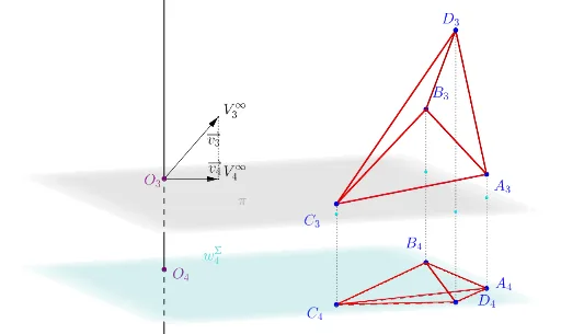
① This example demonstrates graphical models of the projective extension of real 3-space, i.e., the real projective space RP3, visualized in four dimensions, showing points, lines, planes, and surfaces that represent projective geometry concepts including points at infinity and duality. ② Core mathematical concepts include projective geometry, projective spaces, points/lines/planes at infinity, four-dimensional geometric visualization, and incidence/orthogonality relations among geometric objects. ③ Construction highlights: from the construction summary, GeoGebra commands such as Line, Segment, Vector, Ray, Surface, Point, Locus, Plane, Intersect, OrthogonalLine, IntersectPath, Polygon, Sphere, and OrthogonalPlane are used. Objects include O_3, Z_3, A_3, B_3, C_3, D_3 (3D) and A_4, B_4, C_4, D_4, Z_4 (4D), along with vectors like a_3v, b_3v, c_3v, d_3v, a_4v, etc., and surfaces to build the model. ④ Suitable for advanced undergraduate or graduate courses in geometry, projective geometry, or mathematical visualization, and for researchers interested in intuitive understanding of 4D geometry.
GeoGebra Commands & Parameters
Line(O_3, Z_3) → hSegment(A_3, B_3) → iSegment(B_3, C_3) → jSegment(C_3, A_3) → kSegment(A_3, D_3) → lSegment(B_3, D_3) → mSegment(C_3, D_3) → nSegment(A_4, D_4) → qSegment(D_4, B_4) → rSegment(C_4, B_4) → sSegment(C_4, A_4) → tSegment(C_4, D_4) → aSegment(B_4, A_4) → bVector(O_3, Z_3) → z_3vVector(O_3, Z_4) → z_4vVector(O_3, A_3) → a_3vVector(O_3, B_3) → b_3vVector(O_3, C_3) → c_3vVector(O_3, D_3) → d_3vVector(O_3, A_4) → a_4vVector(O_3, B_4) → b_4vVector(O_3, C_4) → c_4vVector(O_3, D_4) → d_4vRay(O_3, A_3) → cRay(O_3, B_3) → dRay(O_3, C_3) → eRay(O_3, D_3) → f_1Ray(O_3, A_4) → h_1Ray(O_3, B_4) → i_1Ray(O_3, C_4) → j_1Ray(O_3, D_4) → k_1Surface((cos(u) * cos(v)), (cos(u) * sin(v)), sin(u), u, (-π), π, v, 0, π) → oSurface((cos(u) * cos(v)), (cos(u) * sin(v)), sin(u), u, (-π), 0, v, 0, π) → uPoint(i) → PAB_3Locus(PAB'_3, PAB_3) → AB'_3Point(j) → PBC_3Locus(PAB'_4, PAB_3) → AB'_4Locus(PBC'_3, PBC_3) → BC'_3Locus(PBC'_4, PBC_3) → BC'_4Point(k) → PAC_3Locus(PAC'_3, PAC_3) → AC'_3Locus(PAC'_4, PAC_3) → AC'_4Point(n) → PCD_3Locus(PCD'_3, PCD_3) → CD'_3Locus(PCD'_4, PCD_3) → CD'_4Point(l) → PAD_3Locus(PAD'_3, PAD_3) → AD'_3Locus(PAD'_4, PAD_3) → AD'_4Point(m) → PBD_3Locus(PBD'_4, PBD_3) → BD'_4Locus(PBD'_3, PBD_3) → BD'_3Plane(A_3, B_3, C_3) → p_1Plane(O_3, p_1) → ξLine(A_3, C_3) → r_1Intersect(r_1, xOyPlane) → W_3OrthogonalLine(W_3, xOyPlane) → s_1Line(A_4, C_4) → t_1Intersect(t_1, s_1) → W_4IntersectPath(ξ, xOyPlane) → a_1Plane(W_4, a_1) → ωSegment(W_3, W_4) → q_1Segment(B_3, B_4) → f_2Segment(A_3, A_4) → g_2Segment(C_3, C_4) → h_2Segment(D_4, D_3) → i_2Polygon(O_3, A_3, C_3) → lineAB_3, r_2, s_2, t_2Polygon(O_3, A_4, C_4) → lineAB_4, j_2, a_2, b_2Polygon(A_3, B_3, C_3) → t1, c_3, k_2, l_2OrthogonalLine(O_3, ξ) → m_2Sphere(O_3, 1) → o_1Intersect(m_2, o_1) → A, BVector(O_3, B) → normalXiOrthogonalLine(O_3, ω) → n_2Intersect(n_2, o_1) → C, DVector(O_3, C) → normalOmegaOrthogonalPlane(O_3, linexyz_1) → linexyzOrthogonalPlane(O_3, linexyw_1) → linexywIntersect(g_2, xOyPlane) → EIntersect(i_2, xOyPlane) → FIntersect(h_2, xOyPlane) → GIntersect(f_2, xOyPlane) → HVector(O_3, I) → fOrthogonalLine(I, xOyPlane) → gIntersect(g, q_2) → JIntersect(g, xOyPlane) → KSegment(I, K) → g_1Vector(O_3, K) → w_1IntersectPath(ω, q_2) → l_1Point(a_1) → LPoint(a_1) → MOrthogonalPlane(L, a_1) → p_2Intersect(l_1, p_2) → NPlane(M, p_2) → p_3Intersect(l_1, p_3) → OIntersectPath(p_2, ξ) → m_1IntersectPath(p_3, ξ) → n_1Polygon(L, M, O, N) → ct1, l_3, m_3, o_2, n_3Intersect(n_1, f_3) → PIntersect(m_1, f_3) → QPolygon(L, M, P, Q) → ct2, l_4, m_4, p_4, q_3Polygon(A_4, B_4, C_4) → t2, c_4, a_4, b_4OrthogonalLine(O_3, t1) → c_1Intersect(c_1, o_1) → R, SVector(O_3, S) → v_1OrthogonalLine(S, p) → d_1Intersect(d_1, p) → TVector(O_3, T) → e_1Segment(S, T) → d_2Ray(O_3, S) → e_2Line(O_3, T) → g_3Ray(O_3, I) → h_3Line(O_3, K) → i_3Line(O_3, linexyz_1) → j_3Line(O_3, linexyw_1) → k_3Intersect(k_3, o_1) → U, VIntersect(j_3, o_1) → W, ZVector(O_3, V) → u_2Vector(O_3, W) → v_2Line(A_3, C_3) → r_3Intersect(r_3, p) → A_1Ray(A_1, C_3) → s_3Line(A_4, C_4) → t_3
AI Drawing Prompt Reference
Create a visualization of the projective extension of real 3-space (real projective space RP3) represented in a four-dimensional view. Start by placing a set of reference points in 3D together with corresponding points in 4D, connect selected point pairs using line-segment edges to form a basic incidence/triangle-like framework in both dimensions. From the same reference point, draw vectors and rays pointing toward the other designated points. Then construct two parametric surfaces resembling spherical parameterizations: use trigonometric expressions with u and v angle parameters, with different u ranges to form two complementary patches. Finally, mark several points derived from the constructed structure and build locus/trajectory relations by linking each marked point to its corresponding primed version along the intended geometric relation, producing the line-generating links associated with the various reference point pairs.
The prompt above was compiled from the original drawing commands and is for reference only.