
Gradient Vector Demonstration
Loading the math board and drawing, please wait…
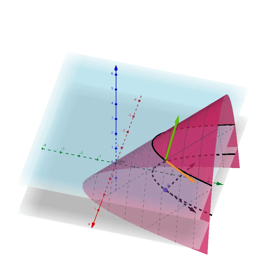
This example demonstrates the geometric meaning of the gradient vector of a function at a point in three-dimensional space. It involves core mathematical concepts such as gradient, vector, 3D function graph, derivative, and unit circle. Key GeoGebra commands used include IntersectPath for finding intersections and Vector for creating vectors, with objects like F, f, G, eq1, A, B, gradfA, u, v, tanv, w, tanw, a. It is suitable for high school and above students studying calculus and vectors to understand the practical application of gradient vectors.
GeoGebra Commands & Parameters
IntersectPath(F, G) → eq1IntersectPath(F, xOyPlane) →IntersectPath(F, xOyPlane) →Vector((-2, 1)) → gradfAVector(A, A + gradfA) → uVector((1, 2)) → vVector(A, A + v) → tanvVector(B, B + tanv) → wVector(B, B + tanw) → a
AI Drawing Prompt Reference
Create a 3D diagram illustrating the geometric meaning of the gradient vector of a function at a point. First, define the intersection of two given objects to determine the relevant base point in space. From this point, draw the gradient-direction vector (using the specified direction) and then create a subsequent vector starting at the same point by extending along the gradient. Add two additional fixed-direction vectors originating from the base point, use one of them to form a “tangential/related direction” vector, and then continue the construction from another corresponding point by translating that direction to create further vectors. The result should visually show how the gradient direction relates to the constructed direction/tangent vectors in 3D.
The prompt above was compiled from the original drawing commands and is for reference only.