
Geometric Interpretation of Pearson's Correlation Coefficient (Draft)
Loading the math board and drawing, please wait…
In collections
Statistical Intuition Builders
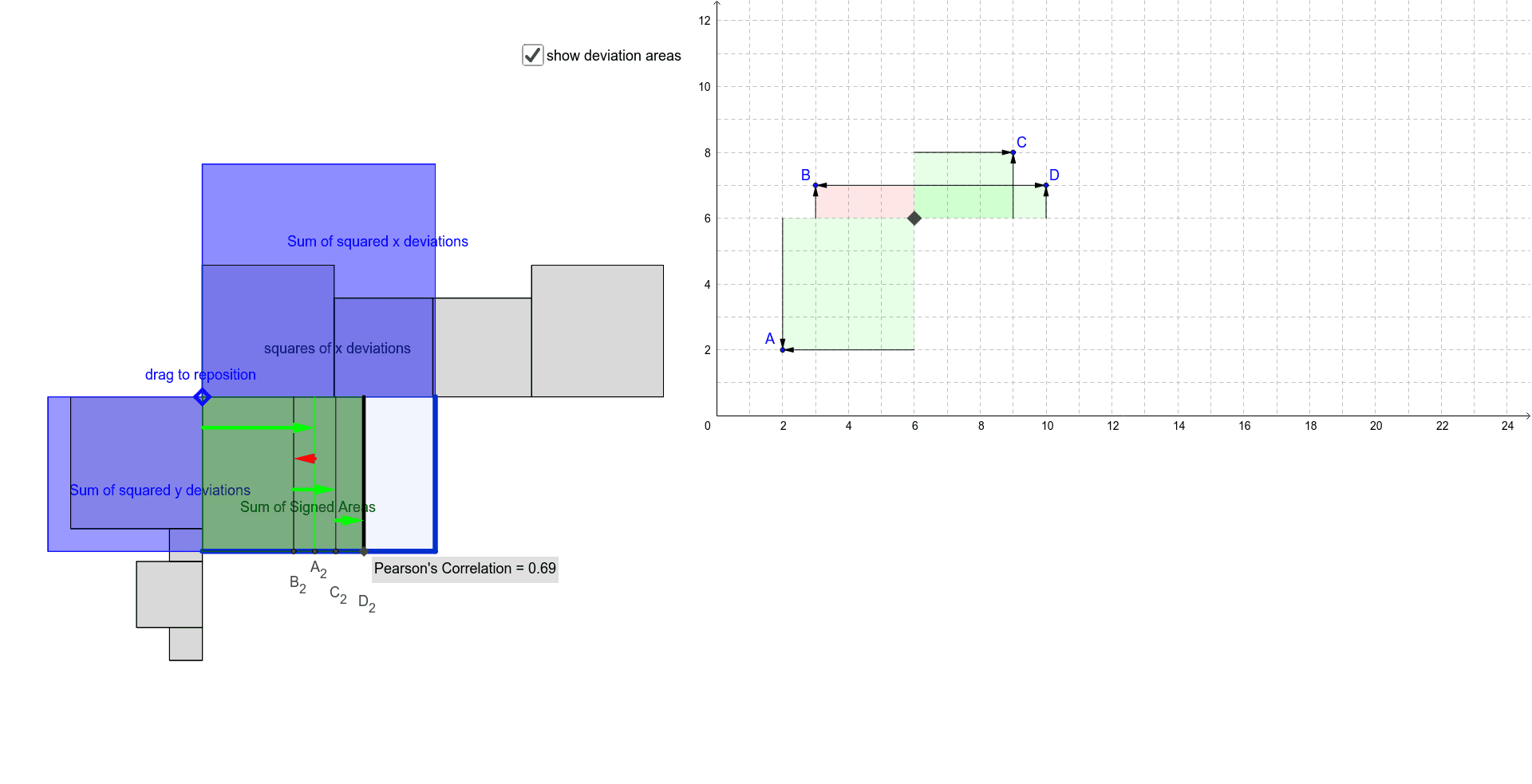
This example attempts to geometrically interpret Pearson's correlation coefficient. It involves core concepts of random variables and correlation. By constructing orthogonal lines, intersections, vectors, polygons, etc., it demonstrates how to calculate and understand the correlation coefficient. Suitable for high school mathematics education and learning.
GeoGebra Commands & Parameters
OrthogonalLine(B, b) → cIntersect(b, c) → EIntersect(a, b) → meanxyOrthogonalLine(C, b) → eOrthogonalLine(D, b) → fOrthogonalLine(B, a) → gOrthogonalLine(A, a) → hOrthogonalLine(A, b) → iOrthogonalLine(C, a) → jOrthogonalLine(D, a) → kIntersect(b, e) → GIntersect(b, f) → HIntersect(b, i) → IIntersect(a, h) → JIntersect(a, g) → KIntersect(a, j) → LIntersect(a, k) → MVector(E, B) → B_xVector(I, A) → A_xVector(G, C) → C_xVector(H, D) → D_xPolygon(B, E, meanxy, K) → poly_B, B_1, e_1, meanxy_1, k_1Polygon(A, I, meanxy, J) → poly_A, a_1, i_1, meanxy_2, j_1Polygon(meanxy, L, C, G) → poly_C, meanxy_3, l_1, c_1, g_1Polygon(meanxy, M, D, H) → poly_D, meanxy_4, m, d_1, h_1Vector(K, B) → B_yVector(J, A) → A_yVector(L, C) → C_yVector(M, D) → D_ySum(signedareas) → SxySum(x({A_x, B_x, C_x, D_x})^(2)) → SxxSum(y({A_y, B_y, C_y, D_y})^(2)) → SyyOrthogonalLine(F, a) → lOrthogonalLine(N, b) → nIntersect(l, n) → OPolygon(meanxy, N, O, F) → poly1, meanxy_5, n_1, o, f_1Line(P, xAxis) → pCircle(P, Segment[meanxy, J]) → qIntersect(q, p, 2) → QCircle(Q, Segment[meanxy, K]) → rIntersect(r, p, 2) → RCircle(R, Segment[meanxy, L]) → sIntersect(s, p, 2) → SCircle(S, Segment[meanxy, F]) → tOrthogonalLine(Q, p) → b_1OrthogonalLine(R, p) → m_1OrthogonalLine(S, p) → p_1Polygon(P, Q, 4) → poly2, r_1, s_1, t_1, a_2, U, VPolygon(Q, R, 4) → poly3, b_2, c_2, d_2, e_2, W, ZPolygon(R, S, 4) → poly4, f_2, g_2, h_2, i_2, A_1, C_1Circle(S, Segment[meanxy, M]) → q_1Intersect(q_1, p, 2) → TOrthogonalLine(T, p) → j_2Polygon(S, T, 4) → poly5, k_2, l_2, m_2, n_2, D_1, E_1Circle(P, u) → p_2Intersect(p_2, p) → F_1, G_1Polygon(P, G_1, 4) → poly6, q_2, r_2, s_2, t_2, H_1, I_1OrthogonalLine(P, p) → a_3Circle(P, Segment[meanxy, I]) → c_3Intersect(c_3, a_3, 1) → J_1Circle(J_1, Segment[meanxy, E]) → d_3Intersect(d_3, a_3, 1) → K_1Circle(K_1, Segment[meanxy, G]) → e_3Intersect(e_3, a_3, 1) → L_1Circle(L_1, Segment[meanxy, H]) → f_3Intersect(f_3, a_3, 1) → M_1Polygon(J_1, P, 4) → poly7, b_3, g_3, h_3, i_3, N_1, O_1Polygon(K_1, J_1, 4) → poly8, j_3, k_3, l_3, m_3, P_1, Q_1Polygon(L_1, K_1, 4) → poly9, n_3, p_3, q_3, r_3, R_1, S_1Polygon(M_1, L_1, 4) → poly10, s_3, t_3, a_4, b_4, T_1, U_1Circle(P, v) → c_4Intersect(c_4, a_3) → V_1, W_1Polygon(V_1, P, 4) → poly11, d_4, e_4, f_4, g_4, Z_1, A_3OrthogonalLine(V_1, a_3) → h_4OrthogonalLine(G_1, h_4) → i_4Intersect(h_4, i_4) → B_3Polygon(V_1, B_3, G_1, P) → poly12, v_1, b_5, g_5, p_4OrthogonalLine(A_2, p) → j_4OrthogonalLine(B_2, p) → k_4OrthogonalLine(D_2, p) → l_4OrthogonalLine(C_2, p) → m_4Intersect(p, j_4) → E_2Intersect(p, k_4) → F_2Intersect(p, m_4) → G_2Intersect(p, l_4) → H_2Polygon(V_1, D_2, H_2, P) → poly13, v_2, d_5, h_5, p_5Mirror(V_1, a_3) → I_2Mirror(D_2, a_3) → J_2Mirror(H_2, a_3) → K_2Mirror(P, a_3) → P'Polygon(I_2, J_2, K_2, P') → poly13', i_5, j_5, k_5, p'Segment(C_2, G_2) → n_4Segment(D_2, H_2) → q_4Segment(A_2, E_2) → r_4Segment(B_2, F_2) → s_4Vector((x(P), y(P) - vecax), (x(A_2), y(P) - vecax)) → wVector((x(A_2), y(P) - vecbx), (x(B_2), y(P) - vecbx)) → u_1Vector((x(B_2), y(P) - veccx), (x(C_2), y(P) - veccx)) → w_1Vector((x(C_2), y(P) - vecdx), (x(D_2), y(P) - vecdx)) → u_2PMCC({A, B, C, D}) → pearcorr
AI Drawing Prompt Reference
Draw a geometric figure to explain Pearson's correlation coefficient. Start by constructing two perpendicular lines b and a, then find intersection points like E and meanxy. Next, construct vectors and polygons such as B_x and A_x. Finally, calculate the components of the correlation coefficient, such as Sxx and Syy.
The prompt above was compiled from the original drawing commands and is for reference only.