
GeoGebra Demo of Logs and Exponential Functions
Loading the math board and drawing, please wait…
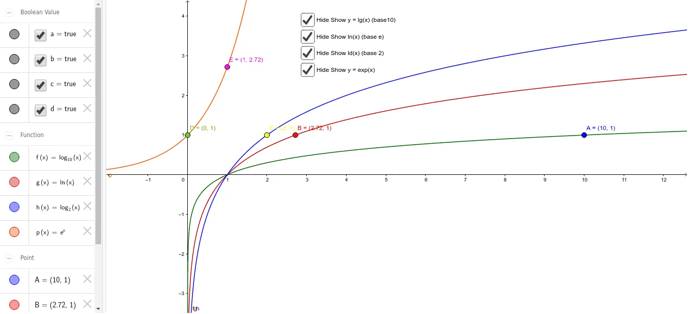
This example dynamically demonstrates the graphs and properties of logarithmic and exponential functions using GeoGebra. It involves core math concepts like exponential functions, logarithmic functions, derivatives, and tangent lines. Key GeoGebra commands used include constructing objects f, g, h, p, A, B, C, D, E, a, b, c, d for graphing functions and tangents. Suitable for high school and above mathematics learners to understand function transformations and properties.
GeoGebra Commands & Parameters
f(x) = lg(x)g(x) = log(x)h(x) = ld(x)p(x) = exp(x)(10, lg(10))(ℯ, log(ℯ))(2, ld(2))(0, exp(0))(1, exp(1))Boolean a(true)Boolean b(true)Boolean c(true)Boolean d(true)
AI Drawing Prompt Reference
Draw a coordinate system containing graphs of logarithmic and exponential functions. Plot three logarithmic curves with bases 10, e, and 2, respectively, and one natural exponential curve. Mark specific points on each logarithmic curve corresponding to their bases, such as (10,1) for base 10, (e,1) for base e, and (2,1) for base 2. On the exponential curve, mark points at x=0 and x=1. Provide four toggles to show or hide each curve for dynamic exploration of function properties.
The prompt above was compiled from the original drawing commands and is for reference only.