
Generating Extreme Point Arrangements on a Sphere
Loading the math board and drawing, please wait…
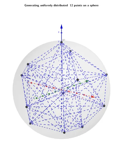
This example demonstrates how to generate extreme point arrangements on a sphere. Key mathematical concepts include vectors, functions, and optimization problems. Using GeoGebra commands such as Sphere, Sequence, and Sum, dynamic generation of points with varying quantities is achieved, allowing observation of their distribution on the sphere. Suitable for high school and above students or teachers for teaching geometric construction and optimization problems.
GeoGebra Commands & Parameters
Sphere((0, 0, 0), R) → d_1Textfield(n) → InputBox2Textfield(i0) → InputBox3Textfield(R) → InputBox1Text(("(up\; to\; 10^{-15})\;\\ accuracy= " * ScientificText[c, 3]), C, true, true) → text8Sequence(Sequence[Segment[Element[lP, k], Element[lP, t]], t, 1, n], k, 1, n) → l1Sum(Zip[UnitVector[A1 - lP(r)], r, B1]) → C1Sum(Zip[UnitVector[A2 - lP(r)], r, B2]) → C2Sum(Zip[UnitVector[A3 - lP(r)], r, B3]) → C3Sum(Zip[UnitVector[A4 - lP(r)], r, B4]) → C4Sum(Zip[UnitVector[A5 - lP(r)], r, B5]) → C5Sum(Zip[UnitVector[A6 - lP(r)], r, B6]) → C6Sum(Zip[UnitVector[A7 - lP(r)], r, B7]) → C7Sum(Zip[UnitVector[A8 - lP(r)], r, B8]) → C8Sum(Zip[UnitVector[A9 - lP(r)], r, B9]) → C9Sum(Zip[UnitVector[A10 - lP(r)], r, B10]) → C10Sum(Zip[UnitVector[A11 - lP(r)], r, B11]) → C11Sum(Zip[UnitVector[A12 - lP(r)], r, B12]) → C12
AI Drawing Prompt Reference
Generate extreme point arrangements on a sphere to demonstrate mathematical concepts like vectors, functions, and optimization. Dynamically create points with varying quantities to observe their distribution. Start by drawing a sphere, then calculate and connect these points to form segments based on input values. Finally, use unit vectors to compute and display the positions of these points on the sphere.
The prompt above was compiled from the original drawing commands and is for reference only.