
General Equations of a Projectile
Loading the math board and drawing, please wait…
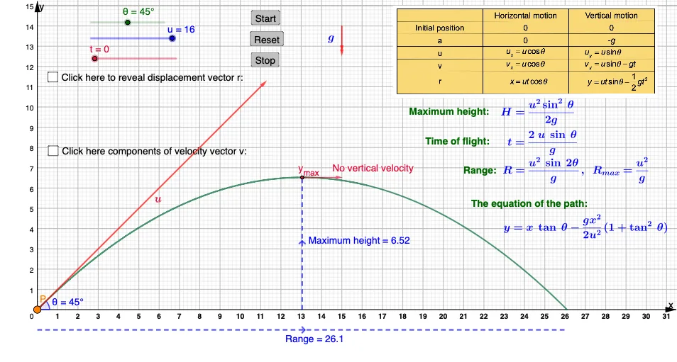
This example demonstrates the trajectory of projectile motion and its general equations through geometric representation. Key math concepts include parametric equations, coordinate geometry, trigonometry, and vectors. Construction highlights involve GeoGebra commands/objects like Vector, Point, Angle, Segment, and Midpoint. Suitable for A-Level Mechanics or introductory university mathematics, helping students understand the derivation and visualization of projectile motion equations.
GeoGebra Commands & Parameters
Vector(((u_1 * cos(θ_1)), (u_1 * sin(θ_1)))) → uPoint(u) → BPoint(u) → CAngle(A, B, C) → θPoint(Circle[E, ((u^(2) * sin((2 * θ)))) / 9.81]) → FSegment(E, F) → gSegment(G, D) → hVector(D, I) → vVector(L, M) → wVector(L, Q) → bVector(P) → dVector(P, (x(P), y(P) + i)) → kVector(P, (x(P) + e, y(P))) → qVector(P, S) → rMidpoint(P, S) → TMidpoint(B, P) → UVector(B, V) → sVector(B, W) → v_1Midpoint(B, V) → ZMidpoint(B, W) → A_1Midpoint(P, (x(P) + e, y(P))) → B_1Midpoint(P, (x(P), y(P) + i)) → C_1
AI Drawing Prompt Reference
Draw the trajectory of a projectile motion, including the initial velocity vector u, starting point A, and endpoint F, gravity acceleration vector g, and velocity vectors v, w, b, d, k, q, r. Use parametric equations to represent the projectile motion, calculate key points using vectors and angles, and finally display the entire motion process.
The prompt above was compiled from the original drawing commands and is for reference only.