
Polar Coordinates by Arwa
Loading the math board and drawing, please wait…
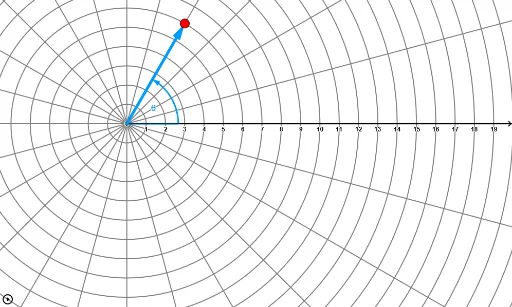
This example demonstrates the plotting and interaction of points, vectors, and curves in polar coordinates. It involves core mathematical concepts such as polar coordinates, vectors, parametric equations, and trigonometry. Key GeoGebra commands used include Vector, CurveCartesian, Line, and Angle, with parameters k, a, r, θ controlling the graphics. Suitable for high school and above students to learn about the polar coordinate system and its applications.
GeoGebra Commands & Parameters
Vector((0, 0), ((r * cos(θ)), (r * sin(θ)))) → rvecCurveCartesian((cos(t) * f(t)), (sin(t) * f(t)), t, 0, (2 * π)) → r1Line(P, (0, 0)) → AngleLineVector((0, 0), (100, 0)) → XvecAngle(Xvec, Vector[If[r > 0, rvec, ((-x(P)), (-y(P)))]]) → PolarAngleAngle(Vector[((-x(P)), (-y(P)))], Vector[P]) → RNegAngle
AI Drawing Prompt Reference
Draw a vector from the origin with length and direction determined by polar coordinates r and θ. Then, draw a line connecting the origin to this vector and calculate the angle between the vector and the positive x-axis. Next, draw a vector of length 100 along the positive x-axis and calculate the angle between it and the previous vector. Finally, plot a parametric curve with x = cos(t) * f(t) and y = sin(t) * f(t) for t ranging from 0 to 2π, showing the shape of the curve in polar coordinates.
The prompt above was compiled from the original drawing commands and is for reference only.