
From Histograms to Frequency Polygons: Area Relationship and Construction
Loading the math board and drawing, please wait…
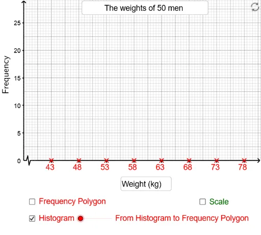
This GeoGebra example demonstrates how to construct a frequency polygon from a histogram and shows how the area enclosed by the frequency polygon relates to the total area of the histogram. Core mathematical concepts include frequency distribution, histograms, frequency polygons, and area equivalence. Construction details: uses CountIf to count frequencies, Midpoint to find class midpoints, PolyLine to connect midpoints, Polygon to create the polygon, Sequence for generating lists, Textfield and RotateText for labels and rotated text, Segment for auxiliary lines, and If for conditional display. Suitable for middle school statistics or introductory college statistics, helping students visualize the equivalence between frequency polygons and histograms.
GeoGebra Commands & Parameters
If(C2 - A2 > 0, C2 - A2 + A3 - C2, 5) → kPoint(Ray[((10 * k), 0), ((10 * k), 1)]) → Q10Point(Ray[((9 * k), 0), ((9 * k), 1)]) → Q9Midpoint(Q10, Q9) → M9Point(Ray[((8 * k), 0), ((8 * k), 1)]) → Q8Midpoint(Q8, Q9) → M8Point(Ray[((7 * k), 0), ((7 * k), 1)]) → Q7Midpoint(Q8, Q7) → M7Point(Ray[((6 * k), 0), ((6 * k), 1)]) → Q6Midpoint(Q6, Q7) → M6Point(Ray[((5 * k), 0), ((5 * k), 1)]) → Q5Midpoint(Q6, Q5) → M5Point(Ray[((4 * k), 0), ((4 * k), 1)]) → Q4Midpoint(Q4, Q5) → M4Point(Ray[((3 * k), 0), ((3 * k), 1)]) → Q3Midpoint(Q3, Q4) → M3Point(Ray[((2 * k), 0), ((2 * k), 1)]) → Q2Midpoint(Q2, Q3) → M2Point(Ray[(k, 0), (k, 1)]) → Q1Midpoint(Q1, Q2) → M1CountIf(x ≠ " ", list7) → nPolygon((unitx, 0.3), (unitx, -0.3), ((2.5 * unitx), -0.3), ((2.5 * unitx), 0.3)) → poly1, a, b, c, dPolyLine((unitx, 0), ((1.5 * unitx), h), ((2 * unitx), (-h)), ((2.5 * unitx), 0)) → eSequence(Segment[(xmin + (xint2 * i), ymax), (xmin + (xint2 * i), ymin)], i, 1, (xmax - xmin) / xint2) → list3Sequence(Segment[(xmin, ymin + (yint2 * i)), (xmax, ymin + (yint2 * i))], i, 1, (ymax - ymin) / yint2) → list4Sequence(Sequence[Segment[((xint2 * (j - 1)) + (xint1 * i), ymax), ((xint2 * (j - 1)) + (xint1 * i), ymin)], i, 1, 4], j, 1, ceil(xmax / xint2)) → list5Sequence(Sequence[Segment[(xmin, ((j - 1) * yint2) + (yint1 * i)), (xmax, ((j - 1) * yint2) + (yint1 * i))], i, 1, 4], j, 1, ceil(ymax / yint2)) → list6Sequence(Segment[((k * i) + (0.5 * k), 0), ((k * i) + (0.5 * k), ((-h)) / 2.5)], i, 1, n - 1) → list9Sequence(Segment[((k * i), 0), ((k * i), ((-h)) / 2.5)], i, 1, n) → list8Textfield(text23) → inputBox2Textfield(text24) → inputBox4Textfield(xint1') → inputBox3Sequence(Polygon[(((i - 0.5) * k), 0), (((i + 0.5) * k), 0), (((i + 0.5) * k), Element[list1, i]), (((i - 0.5) * k), Element[list1, i])], i, 1, n) → list2Segment(Q1, Q2) → l1Segment(Q2, Q3) → l2Segment(Q3, Q4) → l3Segment(Q4, Q5) → l4Segment(Q5, Q6) → l5Segment(Q6, Q7) → l6Segment(Q7, Q8) → l7Segment(Q8, Q9) → l8Segment(Q9, Q10) → l9Sequence(If[y(Element[list10, i]) > y(Element[list11, i - 1]), Rotate[Polygon[Element[list10, i], Element[list11, i - 1], Element[list10, i] - ((0.5 * k), 0)], t, Element[list11, i - 1]], Polygon[Element[list10, i], Element[list10, i] - ((0.5 * k), 0), Element[list10, i]]], i, 2, n) → list2_3Sequence(If[y(Element[list10, i]) < y(Element[list11, i]), Polygon[Element[list10, i], Element[list10, i] - (0, y(Element[list10, i])), Element[list10, i] - ((-0.5 * k), y(Element[list10, i])), Element[list10, i] + ((0.5 * k), 0)], Polygon[Element[list10, i], Element[list11, i], Element[list11, i] - (0, y(Element[list11, i])), Element[list10, i] - (0, y(Element[list10, i]))]], i, 1, n - 1) → list2_2Sequence(If[y(Element[list11, i]) < y(Element[list10, i + 1]), Polygon[Element[list11, i], Element[list10, i + 1], Element[list10, i + 1] - (0, y(Element[list10, i + 1])), Element[list11, i] - (0, y(Element[list11, i]))], Polygon[Element[list10, i + 1], Element[list10, i + 1] - (k / 2, 0), Element[list10, i + 1] - (k / 2, y(Element[list10, i + 1])), Element[list10, i + 1] - (0, y(Element[list10, i + 1]))]], i, 1, n) → list2_1Sequence(If[y(Element[list10, i]) > y(Element[list11, i]), Rotate[Polygon[Element[list10, i], Element[list11, i], Element[list10, i] + ((0.5 * k), 0)], (-t), Element[list11, i]], Polygon[Element[list10, i], Element[list10, i] + ((0.5 * k), 0), Element[list10, i]]], i, 1, n - 1) → list2_4Polygon(Q1, Q1 - ((0.5 * k), 0), Q1 - ((0.5 * k), y(Q1)), (x(Q1), 0)) → poly2, q1, f, i, jPolygon(Element[list10, n], (x(Element[list10, n]), 0), (x(Element[list10, n]) + (0.5 * k), 0), Element[list10, n] + ((0.5 * k), 0)) → poly3, l, m, p, qRotateText("Frequency", 90°) → text12
AI Drawing Prompt Reference
Draw a histogram with a frequency polygon overlaid. Use equal-width class intervals on the x-axis and frequencies on the y-axis. First, draw adjacent rectangular bars with heights proportional to frequencies. Then mark the midpoint of the top edge of each bar, and connect these midpoints with straight line segments to form a polyline. Extend the polyline at both ends to half an interval beyond the outermost midpoints. Show auxiliary shaded regions that illustrate the area equivalence between the frequency polygon and the histogram. Include grid lines and axis labels. The figure should clearly demonstrate the construction from histogram to frequency polygon and the area relationship.
The prompt above was compiled from the original drawing commands and is for reference only.