
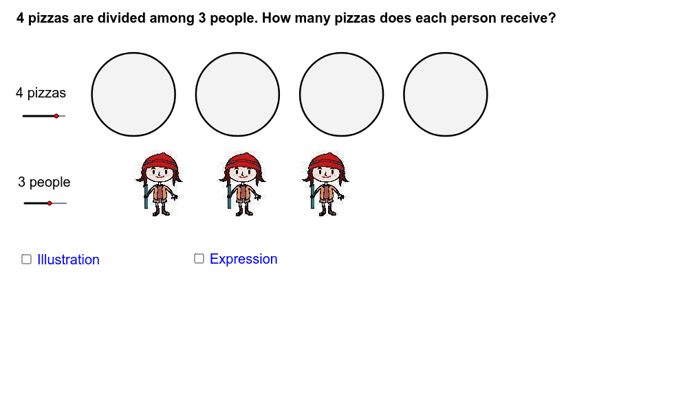
Fraction Division: Partitive Division a ÷ b = a/b Geometric Demonstration
Loading the math board and drawing, please wait…
In collections
Primary School Mathematics Collection
This GeoGebra example visually demonstrates partitive fraction division, showing that a ÷ b equals a/b through an equal-sharing model. Core mathematical concepts include fraction division, partitive division, and the equivalence between division expressions and fractions. The construction uses GeoGebra commands Point, Segment, Sequence, Polygon, and GCD, together with points, segments, polygons, lists, expressions, and text objects to dynamically illustrate the partitioning process. It is suitable for upper elementary and middle school mathematics instruction, classroom demonstrations, lesson planning, and independent student exploration.
GeoGebra Commands & Parameters
Point(Segment[(x(D) + 2 / 5, y(D)), (x(D) + 1, y(D))]) → SSegment(A, (x(A) + 1, y(A))) → l1Point(Segment[(x(A) + 1 / 5, y(A)), (x(A) + 1, y(A))]) → PSegment(B, (x(B) + 1, y(B))) → l2Point(Segment[(x(B) + 2 / 6, y(B)), (x(B) + 1, y(B))]) → QPoint(Segment[(x(C) + 1 / 6 - 0.005, y(C)), (x(Q) - 1 / 6, y(C))]) → RSegment(C, (x(C) + 1, y(C))) → l3Sequence(Circle[((2.5 * (i - 1)), 0), 1], i, 1, a) → list1Sequence(Segment[((2.5 * a), 0), ((2.5 * a) - sin((j * θ)), cos((j * θ)))], j, 1, c - 1) → list2Segment(D, (x(D) + 1, y(D))) → l4Polygon((0.016528925619834656, -3), (1.2165289256198346, -3), (1.2165289256198346, -1.3), (0.016528925619834656, -1.3)) → poly1, e, g, h, iGCD(a, d) → kSegment(A, P) → jSegment(C, R) → lSegment(B, Q) → mSegment(D, S) → nPoint(Segment[(x(A_1) + 1 / 7, y(A_1)), (x(A_1) + 1, y(A_1))]) → P_1Segment(A_1, P_1) → j_1Point(Segment[(x(D_1) + 2 / 5, y(D_1)), (x(D_1) + 1, y(D_1))]) → S_1Point(Segment[(x(A_2) + 1 / 7, y(A_2)), (x(A_2) + 1, y(A_2))]) → P_2GCD(a_1, d_1) → k_1Segment(A_2, P_2) → j_2Segment(D_1, S_1) → n_1Point(Segment[(x(D_2) + 2 / 5, y(D_2)), (x(D_2) + 1, y(D_2))]) → S_2Point(Segment[(x(A_3) + 1 / 7, y(A_3)), (x(A_3) + 1, y(A_3))]) → P_3GCD(a_2, d_2) → k_2Segment(A_3, P_3) → j_3Segment(D_2, S_2) → n_2Sequence(Sequence[CircleSector[(((-1 * f) * sin((((2 * k) - 1) * θ / 2))) + (2.5 * (m - 1)), (f * cos((((2 * k) - 1) * θ / 2)))), (((-1 * f) * sin((((2 * k) - 1) * θ / 2))) - sin(((k - 1) * θ)) + (2.5 * (m - 1)), (f * cos((((2 * k) - 1) * θ / 2))) + cos(((k - 1) * θ))), (((-1 * f) * sin((((2 * k) - 1) * θ / 2))) - sin((k * θ)) + (2.5 * (m - 1)), (f * cos((((2 * k) - 1) * θ / 2))) + cos((k * θ)))], k, 1, 1], m, 1, a) → list4Sequence(Sequence[CircleSector[((f * sin((((2 * k) - 1) * θ / 2))) + (2.5 * (m - 1)), (f * cos((((2 * k) - 1) * θ / 2)))), ((f * sin((((2 * k) - 1) * θ / 2))) + sin((k * θ)) + (2.5 * (m - 1)), (f * cos((((2 * k) - 1) * θ / 2))) + cos((k * θ))), ((f * sin((((2 * k) - 1) * θ / 2))) + sin(((k - 1) * θ)) + (2.5 * (m - 1)), (f * cos((((2 * k) - 1) * θ / 2))) + cos(((k - 1) * θ)))], k, 1, b], m, 1, a) → list3
AI Drawing Prompt Reference
Create a geometric illustration demonstrating the partitive division of fractions, showing that a ÷ b equals a/b. The image should include multiple circles and sectors, visually representing the equal-sharing model of fraction division. Start with a base line, place several circles on it, and then divide each circle into sectors corresponding to the values of a and b. The dynamic display of sector partitioning and combination should intuitively convey the concept of fraction division.
The prompt above was compiled from the original drawing commands and is for reference only.