
Formal Continuity of Functions
Loading the math board and drawing, please wait…
In collections
Fun with Functions
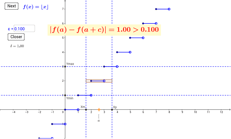
This applet demonstrates the continuity of a function as x approaches a value. Key mathematical concepts include function continuity. Using GeoGebra commands such as Point, Element, If, Max, Textfield, etc., the function's graph is constructed, and its continuity at a specific point is observed. Suitable for high school mathematics education and learning.
GeoGebra Commands & Parameters
Point(xAxis) → SplitPointElement(flist, nf) → gPoint(xAxis) → goalIf((xp ≥ 1) ∧ (xp < 2), 2, xp) → yx8If((xp * xm) ≤ 0, 0, Min[If[xp < 0, (-xp), If[xp ≤ 1, xp^(2), 1]], If[xm < 0, (-xm), If[xm ≤ 1, xm^(2), 1]]]) → ym3Max(If[xm < 0, (-xm), If[xm ≤ 1, xm^(2), 1]], If[xp < 0, 0, If[xp ≤ 1, xp^(2), 1]]) → yx3If(xm ≥ xSplit, y(Max[f_{right}, xm, xp]), If[xp < xSplit, y(Max[f_{left}, xm, xp]), Max[y(Max[f_{left}, xm, xSplit]), y(Max[f_{right}, xSplit, xp])]]) → yx5If(xm ≥ xSplit, y(Min[f_{right}, xm, xp]), If[xp < xSplit, y(Min[f_{left}, xm, xp]), Min[y(Min[f_{left}, xm, xSplit]), y(Min[f_{right}, xSplit, xp])]]) → ym5If((xm ≤ 1) ∧ (xp ≥ 1), Infinity, Max[f_7(xm), f_7(xp)]) → yx7If((xm ≤ 1) ∧ (xp ≥ 1), Infinity, Min[f_7(xm), f_7(xp)]) → ym7If((xm ≤ 0) ∧ (xp ≥ 0), NaN, y(Max[f_9, xm, xp])) → yx9Element(maxlist, nf) → ymaxIf((xm ≤ 0) ∧ (xp ≥ 0), NaN, y(Min[f_9, xm, xp])) → ym9Element(minlist, nf) → yminMax(g(aa) - ymin, ymax - g(aa)) → epsilonTextfield(f_{left}) → inputBox1Textfield(f_{right}) → inputBox2OrthogonalLine(F, xAxis) → aOrthogonalLine(Xm, xAxis) → bOrthogonalLine(Xp, xAxis) → cOrthogonalLine(Ymin, yAxis) → dOrthogonalLine(Ymax, yAxis) → eTextfield(egoal) → inputBox3Polygon(G, C, B, A) → poly1, g_1, c_1, b_1, a_1
AI Drawing Prompt Reference
Draw a graph demonstrating function continuity. Show a piecewise-defined curve on a coordinate plane with a potential discontinuity at a split point. Include a draggable point on the x-axis for the split, and two input boxes for adjusting left and right function expressions. Add vertical dashed lines at sample positions on both sides of the split, and horizontal dashed lines indicating the minimum and maximum function values. Near the split, display a translucent rectangle representing the range of function values, with an adjustable error threshold. The layout is clean, suitable for high school calculus teaching.
The prompt above was compiled from the original drawing commands and is for reference only.