
Forced Harmonic Motion
Loading the math board and drawing, please wait…
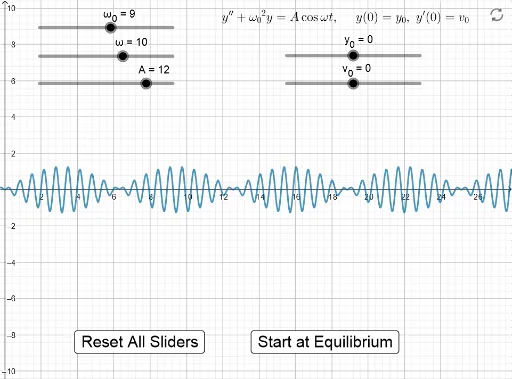
This GeoGebra example visualizes forced harmonic motion, demonstrating the dynamic response of a driven oscillatory system under external periodic forcing. It illustrates core concepts from differential equations, including natural frequency (ω₀), driving frequency (ω), amplitude modulation, phase shift, and energy dissipation. Construction utilizes key objects such as ω, ω₀, y₀, v₀, A, K, y_b, y_r along with differential equation solvers, sliders for parameter control, and dynamic geometric binding to produce an interactive animation. The model is suitable for high school advanced physics, undergraduate calculus, and differential equations courses exploring resonance, frequency response, and oscillatory systems.
GeoGebra Commands & Parameters
Numeric ω(10)Numeric ω_0(9)Numeric y_0(0)Numeric v_0(0)Numeric A(12)A / (ω_0^(2) - ω^(2))y_b(x) = (K * cos((ω * x))) + ((y_0 - K) * cos((ω_0 * x))) + (v_0 / ω_0 * sin((ω_0 * x)))y_r(x) = (((A / ((2 * ω_0)) * x) + v_0 / ω_0) * sin((ω_0 * x))) + (y_0 * cos((ω_0 * x)))