
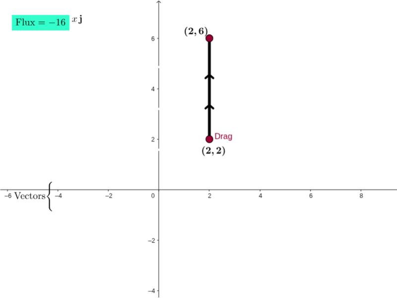
Flux across a line segment demonstration
Loading the math board and drawing, please wait…
This example demonstrates how to calculate the flux of a vector field across a line segment, involving core math concepts like vector fields, line integrals, and flux computation in calculus. It utilizes GeoGebra commands/objects such as Circle, Sequence, Midpoint, Line, CurveCartesian, Derivative, Sum, Point, Ray, Translate, Segment, Sector for construction, suitable for university calculus or physics vector field learning.
GeoGebra Commands & Parameters
Circle((0, 0), 16) → kSequence(Sequence[Vector[(j, k), (j + (scale * F_1(j, k)), k + (scale * F_2(j, k)))], j, xmin, xmax, xstep], k, ymin, ymax, ystep) → vFieldSequence(((x(Element[inicialPts, i]) * cos((w * time))) - (y(Element[inicialPts, i]) * sin((w * time))), (x(Element[inicialPts, i]) * sin((w * time))) + (y(Element[inicialPts, i]) * cos((w * time)))), i, 1, 8) → particlesListSequence(CurveCartesian[(x(Element[inicialPts, i]) * cos((w * t))) - (y(Element[inicialPts, i]) * sin((w * t))), (x(Element[inicialPts, i]) * sin((w * t))) + (y(Element[inicialPts, i]) * cos((w * t))), t, 0, time], i, 1, 8) → pathlinesListCircle(divPt, 0.5) → divGlowCircleSequence(Segment[Rotate[curlPt - (0.5, 0), k + curlAngle, curlPt], Rotate[curlPt + (0.5, 0), k + curlAngle, curlPt]], k, 0, 2.0944, 1.0472) → spokesMidpoint(I, J) → MidPointLine(K, xAxis) → gLine(L, xAxis) → hLine(M, xAxis) → iCurveCartesian((t * x(J)) + ((1 - t) * x(I)), (t * y(J)) + ((1 - t) * y(I)), t, 0, 1) → pathTestCurveCartesian(x(pathTest(i)), y(pathTest(i)), i, 0, s) → partPathTestDerivative(pathTest) → DpathSum(Sequence[(((F_1(x(pathTest(i + dS / 2)), y(pathTest(i + dS / 2))), F_2(x(pathTest(i + dS / 2)), y(pathTest(i + dS / 2)))) * (y(Dpath(i + dS / 2)), (-x(Dpath(i + dS / 2))))) * dS), i, 0, s - dS, dS]) → FluxTestSequence(Vector[pathTest(i), pathTest(i) + ((scale * F_1(x(pathTest(i)), y(pathTest(i)))), (scale * F_2(x(pathTest(i)), y(pathTest(i)))))], i, 0, s, 0.25) → PathVectorsPoint(k) → PRay((0, 0), N) → dTranslate(normalvector_1, PtPath_1) → uSegment(pathTest(0.3), pathTest(0.3 + 0.01)) → arrow1Segment(pathTest(0.6), pathTest(0.6 + 0.01)) → arrow2Sector(k, Q, N) → p