
First Order ODE Visualization
Loading the math board and drawing, please wait…
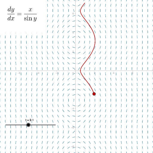
This example demonstrates the solution of first-order ordinary differential equations (ODEs), slope fields, and integration areas through graphical methods. Key mathematical concepts include ODEs, slope fields (SlopeField), numerical integration (numericalIntegral1), and polygons (Polygon). The construction utilizes GeoGebra commands like SolveODE for solving ODEs, SlopeField for plotting direction fields, and Polygon for generating integration regions, involving objects such as A, t, B, C, a, b, c, d, D, E. Suitable for high school students and beginners in differential equations.
GeoGebra Commands & Parameters
SolveODE(x, sin(y), x(A), y(A), t, 0.1) → numericalIntegral1SlopeField(x / sin(y), 30, 0.5) → slopefield1Polygon(B, C, 4) → poly1, a, b, c, d, D, E
AI Drawing Prompt Reference
Visualize the solution of a first-order ordinary differential equation, slope fields, and integration areas, showing the numerical solution, direction field, and integration polygon, start by drawing a polygon formed by four points, then plot arrows to represent the slope field, and finally display the numerical solution of the differential equation as a curve, ensuring all elements are clearly distinct and interconnected.
The prompt above was compiled from the original drawing commands and is for reference only.