
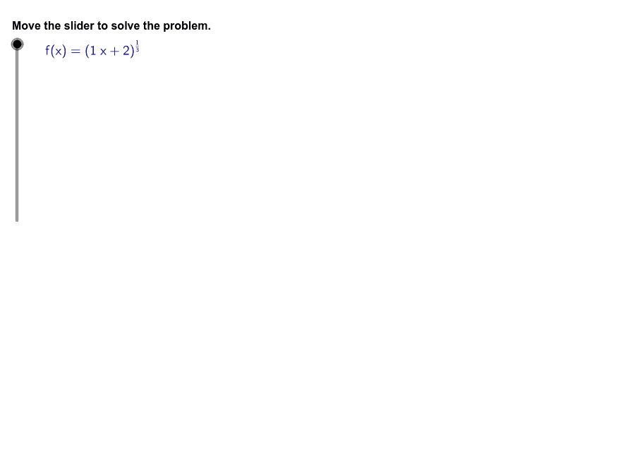
Finding the Inverse of the Cube Root Function f(x)=∛(x+2)
Loading the math board and drawing, please wait…
In collections
CCGPS AA Unit 6 Lesson 7
This example demonstrates how to find the inverse of the radical function f(x)=∛(x+2) and visualizes the symmetry of the function and its inverse about the line y=x. Core concepts include radical functions, definition and existence of inverse functions, domain–range interchange, and reflection transformations. Construction uses LaTeX for formula rendering, Simplify for algebraic simplification, If for conditional logic, TableText for step‑by‑step tables; sliders (stepper, steps, counter) drive animation, buttons (button1, button2) provide interaction, a mirror object creates the y=x reflection, and objects inversefront, inversemid, inversefunc represent stages of the inverse graph. Suitable for high‑school algebra or college‑prep courses as a teaching demo, self‑study tool, or exam review material.
GeoGebra Commands & Parameters
LaTeX(steps) → counterSimplify(((a * x) + b)^(1 / 3)) → fLaTeX((("\textcolor{#000099}{f(x)=" * f) * "}")) → ProblemLaTeX((("\text{Since the inverse function results from switching the input and output variables}\cr\text{of the original function, identify which variable represents the input and which}\cr\text{represents the output. For the function }\textcolor{#000099}{f(x) = " * f) * "}\text{, }\textcolor{#000099}{x}\text{ is the input (independent)}\cr\text{variable, and }\textcolor{#000099}{f(x)}\text{ is the output (dependent) variable. Therefore, swap }\textcolor{#000099}{f(x)}\text{ and }\textcolor{#000099}{x}.")) → text2LaTeX("\text{Determine the domain of }\textcolor{#000099}{f(x)}.") → text16LaTeX("\text{Determine whether the function }\textcolor{#000099}{f(x)}\text{ exhibits one-to-one correspondence.}") → text18LaTeX("\text{Determine the range of }\textcolor{#000099}{f(x)}.") → text21LaTeX("\text{Match domains to ranges to find the inverse(s) of }\textcolor{#000099}{f(x)}.") → text23LaTeX("\text{Check that the range of }\textcolor{#000099}{f(x)}\text{ matches the domain of }\textcolor{#006633}{g(x)}.") → text25Simplify((x^(3) - b) / a) → gLaTeX("\text{Switch the domain and function variables, and then rename }\textcolor{#000099}{f(x)}\text{ as }\textcolor{#006633}{f^{-1}(x).}") → text1LaTeX("\text{Next, rename }\textcolor{#000099}{f(x)}\text{ as }\textcolor{#006633}{f^{-1}(x)}\text{, since this new relation represents the inverse of the}\cr\text{original function.}") → text4If(a ≟ 1, LaTeX["f^{-1}(x)"], If[a ≟ -1, LaTeX["-f^{-1}(x)"], LaTeX[(a * "f^{-1}(x)")]]) → inversefrontIf(b ≟ 0, LaTeX[""], If[b < 0, LaTeX[("-" * abs(b))], LaTeX[("+" * abs(b))]]) → inversemidIf(a ≟ 1, LaTeX[(("\sqrt[3]{f^{-1}(x)" * inversemid) * "}")], If[a ≟ -1, LaTeX[(("\sqrt[3]{-f^{-1}(x)" * inversemid) * "}")], LaTeX[(((("\sqrt[3]{" * a) * "f^{-1}(x)") * inversemid) * "}")]]) → inversefuncLaTeX((((("\text{The resulting inverse relation, }\textcolor{#006633}{x = " * inversefunc) * "}\text{, is the possible inverse function of}\cr\text{the original function. It must be evaluated to determine whether it has }\cr\text{one-to-one correspondence with the original function, }\textcolor{#000099}{f(x) = ") * f) * "}.")) → text6LaTeX("f(x)") → inversefrontaIf(b ≟ 1, LaTeX["f(x)"], If[b ≟ -1, LaTeX["-f(x)"], LaTeX[(b * "f(x)")]]) → inversemidaIf(a ≟ 1, LaTeX[(("\sqrt[3]{f(x)" * inversemid) * "}")], If[a ≟ -1, LaTeX[(("\sqrt[3]{-f(x)" * inversemid) * "}")], LaTeX[(((("\sqrt[3]{" * a) * "f(x)") * inversemid) * "}")]]) → inversefuncaLaTeX("\text{Solve the possible inverse for }\textcolor{#006633}{f^{-1}(x)}.") → text7LaTeX("\text{Determine the domain of }\textcolor{#006633}{f^{-1}(x)}.") → text9LaTeX("\text{Determine the range of }\textcolor{#006633}{f^{-1}(x)}.") → text13LaTeX("\text{We need to compare the range of }\textcolor{#006633}{f^{-1}(x)}\text{ to the domain of }\textcolor{#000099}{f(x)}.") → text14LaTeX("\text{The function }\textcolor{#000099}{f(x)}\text{ can only have an inverse over the parts of its domain where it exhibits}\cr\text{one-to-one correspondence.}") → text19LaTeX("\text{The function }\textcolor{#006633}{f^{-1}(x)}\text{ is a polynomial function so its domain is all real numbers.}") → text11LaTeX("\text{The range of }\textcolor{#000099}{f(x)}\text{ is }\textcolor{#000099}{(-\infty,+\infty)}\text{. The domain of }\textcolor{#006633}{f^{-1}(x)}\text{ is }\textcolor{#006633}{(-\infty,+\infty)}.") → text26LaTeX("\text{Check that }\textcolor{#000099}{f(x)}\text{ is one-to-one with the horizontal line test.}") → text27LaTeX("\text{Check that }\textcolor{#006633}{f^{-1}(x)}\text{ is a function using the vertical line test.}") → text28LaTeX((((("\text{The inverse of }\textcolor{#000099}{f(x)=" * f) * "}\text{ is }\textcolor{#006633}{f^{-1}(x)=") * g) * "}.")) → text29LaTeX((("\text{We can determine that the function }\textcolor{#000099}{f(x) =" * f) * "}\text{ does show one-to-one}\cr\text{correspondence for all domain values by noting that cube roots, and other odd roots,}\cr\text{preserve negative signs so that no two values of }\textcolor{#000099}{x}\text{ can produce the same }\textcolor{#000099}{f(x)}\text{ value.}")) → text20LaTeX("\text{Use the buttons below to return to the original problem or}\cr\text{randomly generate a similar practice problem.}") → text31TableText({{LaTeX[(("\textcolor{#000099}{x=" * inversefunca) * "}")], LaTeX["\text{Equation with variables switched}"]}, {LaTeX[(("\textcolor{#006633}{x=" * inversefunc) * "}")], LaTeX["\text{Rename }\textcolor{#000099}{f(x)}\text{ as }\textcolor{#006633}{f^{-1}(x)}."]}}) → text5TableText({{LaTeX[(("\textcolor{#000099}{f(x)=" * f) * "}")], LaTeX["\text{Original function}"]}, {LaTeX[(("\textcolor{#000099}{x=" * inversefunca) * "}")], LaTeX["\text{Switch }\textcolor{#000099}{f(x)}\text{ and }\textcolor{#000099}{x}."]}}) → text3LaTeX("\text{In other words, the domain of }\textcolor{#006633}{f^{-1}(x)} \text{ is }\textcolor{#006633}{(-\infty,+\infty)}.") → text12TableText({{LaTeX[(("\textcolor{#006633}{x=" * inversefunc) * "}")], LaTeX["\text{Possible inverse}"]}, {LaTeX[(((("\textcolor{#006633}{x^3=(" * a) * ")f^{-1}(x)+(") * b) * ")}")], LaTeX["\text{Cube both sides.}"]}, {LaTeX[(((("\textcolor{#006633}{" * Simplify[x^(3) - b]) * "=(") * a) * ")f^{-1}(x) }")], LaTeX[(("\text{Subtract }\textcolor{#006633}{" * b) * "}\text{ from both sides.}")]}, {LaTeX[(((("\textcolor{#006633}{\frac{" * Simplify[x^(3) - b]) * "}{") * a) * "}=f^{-1}(x)}")], LaTeX[(("\text{Divide both sides by }\textcolor{#006633}{" * a) * "}.")]}, {LaTeX[(("\textcolor{#006633}{f^{-1}(x)=" * g) * "}")], LaTeX["\text{Simplify and use the Symmetric Property of Equality.}"]}}) → text8LaTeX("\text{We need to know where }\textcolor{#006633}{f^{-1}(x)}\text{ is defined in order to know its domain, which we}\cr\text{want to compare to the range of }\textcolor{#000099}{f(x)}.") → text10LaTeX("\text{There are no limitations on the output values; therefore, the range of }\textcolor{#006633}{f^{-1}(x)}\text{ is }\cr\textcolor{#006633}{(−\infty, +\infty)}.") → text15LaTeX("\text{There are no limitations on the input values; therefore, the domain }\text{of }\textcolor{#000099}{f(x)}\text{ is }\textcolor{#000099}{(−\infty, +\infty)}.") → text17LaTeX("\text{There is no limitation on the values }\textcolor{#000099}{f(x)}\text{ can have, so its range is }\textcolor{#000099}{(-\infty,+\infty)}.") → text22TableText({{LaTeX["\text{Domain of }\textcolor{#000099}{f(x)}\text{:}"], LaTeX["\text{Inverse function with matching range:}"]}, {LaTeX["\textcolor{#000099}{(-\infty,+\infty)}"], LaTeX[(("\textcolor{#006633}{f^{-1}(x)=" * g) * "}")]}}) → text24
AI Drawing Prompt Reference
Create a coordinate plane with the cube root function f(x)=³√(x+2) graphed in blue and its inverse function graphed in green, showing symmetry about the y=x line. Include the y=x mirror line, colored LaTeX formulas for the functions, step-by-step tables illustrating variable swapping and the inverse calculation process, slider controls for animating through steps, and interactive buttons. Mark both the domain and range of the function and its inverse as all real numbers (-∞, +∞).
The prompt above was compiled from the original drawing commands and is for reference only.