
Find the Rolling Function
Loading the math board and drawing, please wait…
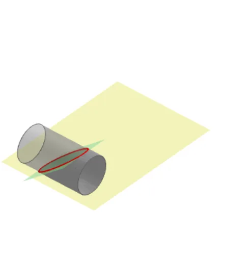
This example demonstrates how to use the sine function to simulate the rolling of an object. Key mathematical concepts include the properties of the sine function and its application in practical problems. Using GeoGebra commands such as Intersect, Segment, Polygon, etc., a dynamic graphical representation of the object's rolling can be constructed. Suitable for high school mathematics education and learning.
GeoGebra Commands & Parameters
Intersect(xAxis, zAxis) → OSegment(O, E) → fPolygon((-4, -4, 0), (((2 * π) * r) + 4, -4, 0), (((2 * π) * r) + 4, h + 4, 0), (-4, h + 4, 0)) → v2, p, q, s, tCylinder(M_1, M_2, r) → b, d, e_1, gPlane(M, N, P) → eLine(M_2, M_1) → jSequence(Segment[Rotate[O, i°, j], Rotate[E, i°, j]], i, 0, 359) → LmSequence(Rotate[O, i°, j], i, 0, 359) → LpuPolygon(M, N, P, Q) → v4, m_1, n_1, p_1, q_1Line((abw, 0, r), (abw, h, r)) → dreRotate(J, o°, dre) → J'Circle(dre, J) → kTranslate(g, Vector[J]) → g'Segment(K, J') → mSegment(O, J) → nSegment(J', R) → cRay(((π * r / 2), 0), ((π * r / 2), 1)) → i_1Ray((((3 / 2 * π) * r), 0), (((3 * π) * r / 2), 1)) → h_1Textfield(af) → Eingabefeld1Textfield(bf) → Eingabefeld2Textfield(cf) → Eingabefeld3Textfield(df) → Eingabefeld4Sequence(Intersect[Element[Lm, i], v4], i, 1, 360) → L_1Sequence(Segment[Element[Lpu, i], Element[L_1, i]], i, 1, 360) → L_2Sequence(Rotate[J', i°, dre], i, 0, 359) → L_3Rotate(J, -1°, dre) → J'_1CircumcircleArc(J, J'_1, J') → c_1Cylinder(Mru, Mro, r) → u, d_1, k_1, vSequence((((π * r / 180) * i), 0, 0), i, 0, 359) → LxSequence(Translate[Element[L_2, i], Vector[Element[L_1, i], Element[Lx, i]]], i, 1, o) → L_4Mirror(L_4, xAxis) → L_5Sequence(Rotate[J', i°, dre], i, 0, 359) → L_8Sequence(Translate[Element[L_2, i], Vector[Element[L_1, i], Element[L_8, i]]], i, 2, 360 - o) → L_7Mirror(L_7, w) → L_9Sequence((x(Element[L_8, i]), y(Element[L_1, i]), z(Element[L_1, i])), i, 360 - o, 360) → L_{10}Segment(J, J + (0, h, 0)) → l_1Textfield(r) → Eingabefeld5Sequence((x(Element[Lx, i]), y(Element[L_1, i]), 0), i, 1, o - 2) → L_6Sequence(π / 2 + ((i * 2) * π), i, 1, 100) → L_{11}Ray((((2 * π) * r), 0), (((2 * π) * r), 1)) → g_1Ray(S, S + (0, 1)) → r_1