
Filling a Container at Constant Rate
Loading the math board and drawing, please wait…
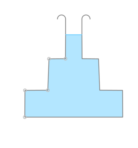
This example demonstrates the process of filling a container at a constant rate, visually representing the rising water level through dynamic graphs. Core mathematical concepts include function graphing, logical reasoning, geometric diagram construction, division, median value calculation, and prism volume computation. Key GeoGebra commands and objects used, as derived from the construction summary, are PointIn, Polygon, Point, Mirror, If, Arc, Join, Min, PolyLine, Intersect, Segment, and RotateText, enabling precise dynamic water surface and container visualization. Suitable for high school mathematics education, covering function graphs, geometric volumes, and dynamic geometric constructions.
GeoGebra Commands & Parameters
PointIn((x ≤ 2.5) ∧ (x ≥ 0.01) ∧ (y ≥ 0.01) ∧ (y ≤ 5)) → A2Polygon(Join[{Reverse[A1:A5], B1:B5}]) → poly5'Polygon(Join[{Reverse[A1:A3], B1:B3}]) → poly3'Point(Segment[(0, 0), (3, 0)]) → A1Mirror(A1, x = 3) → B1PointIn((x ≤ 2.49) ∧ (x ≥ 0) ∧ (y ≥ y(A2) + 0.01) ∧ (y ≤ 5.01)) → A3PointIn((x ≤ 2.5) ∧ (x ≥ 0.01) ∧ (y ≥ y(A3) + 0.01) ∧ (y ≤ 5.02)) → A4PointIn((x ≤ 2.49) ∧ (x ≥ 0) ∧ (y ≥ y(A4) + 0.01) ∧ (y ≤ 5.03)) → A5Mirror(A5, x = 3) → B5Mirror(A4, x = 3) → B4Mirror(A3, x = 3) → B3Mirror(A2, x = 3) → B2Mirror(A6, x = 3) → B6Polygon(A6, A5, B5, B6, A4, A3, A2, A1, B1, B2, B3, B4) → poly6, a6, b4_1, b5, b6, a5, a4_1, a3_1, a2_2, a1_3, b1_3, b2_2, b3_1Polygon(Join[{Reverse[A1:A2], B1:B2}]) → poly2'Polygon(Join[{Reverse[A1:A4], B1:B4}]) → poly4'If(t < C1, 0, 1) → hArc(Circle[A7, A8, A9], A7, A9) → cMirror(A7, x = 3) → B7Mirror(A7, x = 3) → A7'Mirror(A9, x = 3) → A9'Arc(Mirror[Circle[A7, A8, A9], x = 3], A7', A9') → c'Join({Reverse[A7:A1], B1:B7}) → list1Min(5.04, If[t < C1, (-3 + x(A1) + sqrt((3 - x(A1))^(2) + ((t * poly6) * ((-x(A2)) + x(A1)) / (y(A2) - y(A1))))) / (((-x(A2)) + x(A1)) / (y(A2) - y(A1))), If[t < C2, y(A2) + (-3 + x(A2) + sqrt((3 - x(A2))^(2) + (((t - C1) * poly6) * ((-x(A3)) + x(A2)) / (y(A3) - y(A2))))) / (((-x(A3)) + x(A2)) / (y(A3) - y(A2))), If[t < C3, y(A3) + (-3 + x(A3) + sqrt((3 - x(A3))^(2) + (((t - C2) * poly6) * ((-x(A4)) + x(A3)) / (y(A4) - y(A3))))) / (((-x(A4)) + x(A3)) / (y(A4) - y(A3))), If[t < C4, y(A4) + (-3 + x(A4) + sqrt((3 - x(A4))^(2) + (((t - C3) * poly6) * ((-x(A5)) + x(A4)) / (y(A5) - y(A4))))) / (((-x(A5)) + x(A4)) / (y(A5) - y(A4))), y(A5) + (-3 + x(A5) + sqrt((3 - x(A5))^(2) + (((t - C4) * poly6) * ((-x(A6)) + x(A5)) / (y(A6) - y(A5))))) / (((-x(A6)) + x(A5)) / (y(A6) - y(A5)))]]]]) → aPolyLine(list1) → gIntersect(f, g) → A, BPolygon(A, A1, B1, B) → poly1, a_1, a1, b1, bPolygon(A, A2, A1, B1, B2, B) → poly2, a_2, a2, a1_1, b1_1, b2, b_1Polygon(A, A3, A2, A1, B1, B2, B3, B) → poly3, d, e, f_1, g_1, h_1, i_1, j_1, k_1Polygon(A, A4, A3, A2, A1, B1, B2, B3, B4, B) → poly4, a_3, b_2, a4, a3, a2_1, a1_2, b1_2, b2_1, b3, b4Segment(A, B) → l_1Polygon(A, A5, B5, B, A4, A3, A2, A1, B1, B2, B3, B4) → poly5, i, s, m_1, n_1, j, k, l, m, n, p, q, rRotateText(text1, 90°) → text3
AI Drawing Prompt Reference
Draw a dynamic process of a container being filled with water, showing the rising water level with function graphs. The container is a symmetrical cylinder with five points from left to right at the bottom. The water level rises gradually from left to right, represented by different colored polygons for the water surface and container. The water surface is connected by arcs, and its height changes over time, shown by function graphs. Lines connect the water surface to the container, dynamically displaying the rising process of the water level.
The prompt above was compiled from the original drawing commands and is for reference only.