
Comparing Binomial and Normal Distributions
Loading the math board and drawing, please wait…
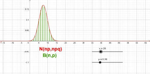
① This example dynamically illustrates how the binomial distribution approximates the normal distribution as the number of trials increases, showing the convergence of discrete probability masses to a continuous bell-shaped curve. ② Core mathematical concepts include binomial distribution, normal distribution, central limit theorem, probability mass/density functions, and cumulative distributions. ③ Construction highlights: the GeoGebra Sequence command generates the binomial probability values, sliders control parameters n (number of trials) and p (success probability), a normal curve is overlaid for comparison, and text objects display key statistics. ④ Suitable for high school to undergraduate statistics courses, this interactive tool helps students visualize the central limit theorem, explore the effects of parameter changes on approximation accuracy, and bridge the gap between discrete and continuous probability models.
GeoGebra Commands & Parameters
Sequence(Segment[(k, 0), (k, ((nCr[n, k] * p^(k)) * (1 - p)^(n - k)))], k, 0, n) → l1
AI Drawing Prompt Reference
Create a statistical chart comparing binomial and normal distributions. Draw vertical line segments from the x-axis upward to represent binomial probability masses at integer trial counts, forming a discrete bar-like outline. Overlay a smooth normal distribution curve that approximates the discrete shape. Include two sliders to adjust the number of trials and success probability, so that increasing trials makes the discrete bars converge to the continuous curve, illustrating the central limit theorem. Display key statistics such as mean and variance as text labels. The layout should be clean and suitable for educational demonstration.
The prompt above was compiled from the original drawing commands and is for reference only.