
Factor and Remainder Theorem Demo
Loading the math board and drawing, please wait…
In collections
Grade 12 Calculus & Vectors MCV4U1
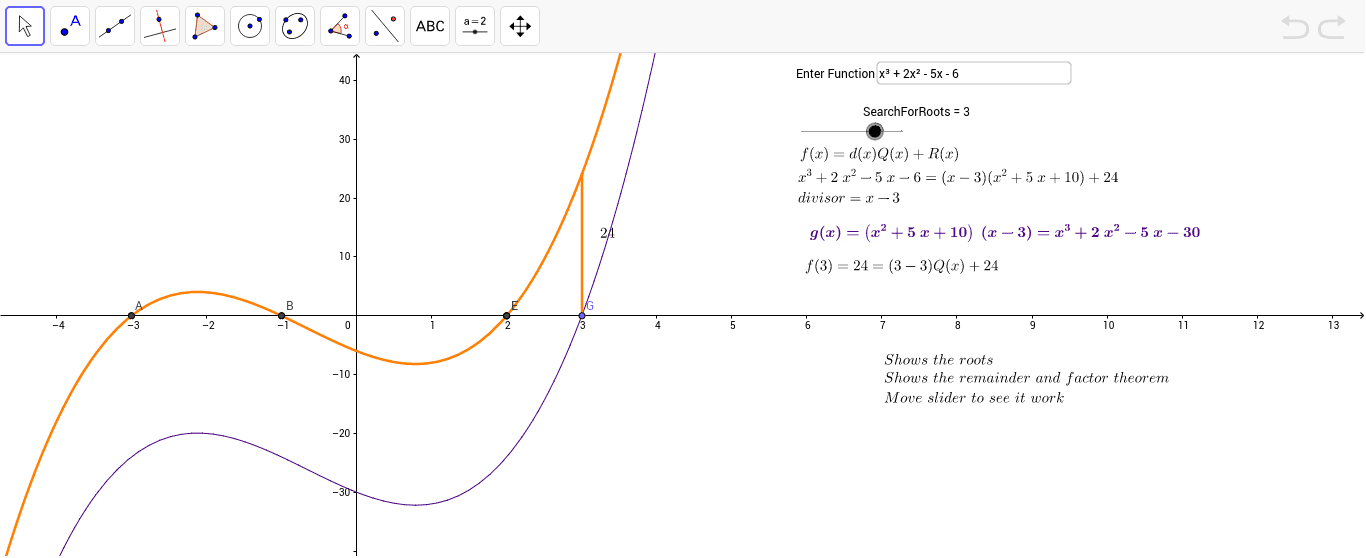
① This example demonstrates how to apply the Factor and Remainder Theorems to find polynomial zeros and illustrate polynomial division. ② Core concepts include polynomial factorization, the Remainder Theorem, root determination, and the graph of a polynomial function. ③ Construction highlights: Intersect to locate axis intercepts, Division for polynomial long division, Root to compute zeros, Min/Max to mark extrema, Point, Vector, Segment for auxiliary geometry, and Textfield/inputBox1 for interactive input. ④ Suitable for high‑school algebra and pre‑calculus courses, as well as introductory college mathematics review.
GeoGebra Commands & Parameters
Intersect(f, y = 0) → A, B, ETextfield(f) → inputBox1Division(f, x - SearchForRoots) → list1Min({Root[f]}) → aRoot(f) → C, D, FMin(x(list2)) → bMax(x(list2)) → cPoint(xAxis) → GVector(G, H) → uVector(G, I) → vSegment(H, I) → dSegment(G, I) → eSegment(G, H) → hSegment(G, I) → i
AI Drawing Prompt Reference
Draw a polynomial function graph, find its intersections with the x-axis at points A, B, and E, use inputBox1 to input the polynomial expression, perform polynomial division to get the quotient and remainder, mark the zeros of the polynomial at points C, D, and F, find the minimum value a and maximum value b of the function, plot point G on the x-axis, draw vectors u and v from G to H and I, draw line segment d between H and I, draw line segment e between G and I, draw line segment h between G and H, and draw line segment i between G and I.
The prompt above was compiled from the original drawing commands and is for reference only.