
Extraction, Frequencies and Probabilities of a Ballot Box
Loading the math board and drawing, please wait…
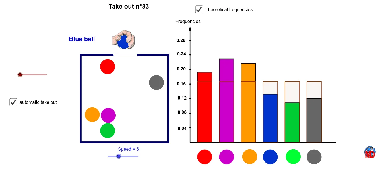
This GeoGebra example demonstrates the relationship between empirical frequencies and theoretical probabilities when drawing balls from a three-dimensional ballot box (cuboid). It visually shows how the observed frequency of each outcome converges to the theoretical probability as the number of trials increases, illustrating the law of large numbers. Core concepts include probability, frequency, hypothesis testing, exponential functions, and 3D geometry with vectors. The construction uses commands such as Polygon, Circle, Sequence, First, CountIf, Element, Point, Segment, and Vector to build the cuboid, balls, and dynamic counters. A slider (Speed) controls the number of extractions, and the interface displays frequency counts and probability comparisons. Suitable for high school or introductory college statistics courses, this interactive tool helps students grasp the difference between empirical and theoretical probability and supports discussions on hypothesis testing and random sampling.
GeoGebra Commands & Parameters
Polygon(E, F, 4) → poly1, e_1, f_1, h, i, G, HCircle(C, 1) → k_1Circle(A, 1) → pCircle(AA, 1) → tCircle(I, 1) → c_1Circle(M, 1) → d_1Circle(J, 1) → g_1Sequence(Random[1, 6], i, 1, 1000) → liste1First(liste1, n) → TirageCountIf(x ≟ 1, Tirage) → B3CountIf(x ≟ 2, Tirage) → B4CountIf(x ≟ 3, Tirage) → B5CountIf(x ≟ 4, Tirage) → B6CountIf(x ≟ 5, Tirage) → B7CountIf(x ≟ 6, Tirage) → B8Element(liste1, n) → ddCircle(O, 1) → eCircle(O, 1) → fCircle(O, 1) → gCircle(O, 1) → qCircle(O, 1) → rCircle(O, 1) → sPoint(h) → PPoint(h) → QSegment(P, Q) → jSegment(R, S) → mSegment(R, T) → a_1Point(m) → UPoint(m) → VPoint(m) → WPoint(m) → ZPoint(m) → A_1Point(m) → B_1Point(m) → C_1Point(m) → D_1Point(m) → E_1Point(m) → F_1Polygon(U, V, I_1, G_1) → poly2, u, v, i_1, g_2Polygon(W, J_1, K_1, Z) → poly3, w, j_1, k_2, zPolygon(A_1, B_1, M_1, L_1) → poly4, a_2, b_1, m_1, l_1Polygon(N_1, O_1, D_1, C_1) → poly5, n_1, o_1, d_2, c_2Point(m) → P_1Point(m) → Q_1Polygon(E_1, F_1, S_1, R_1) → poly6, e_2, f_2, s_1, r_1Polygon(P_1, Q_1, U_1, T_1) → poly7, p_1, q_1, u_1, t_1Point(a_1) → H_1Point(a_1) → V_1Point(a_1) → W_1Point(a_1) → Z_1Point(a_1) → A_2Point(a_1) → B_2Point(a_1) → C_2Vector(R, T) → v_1Polygon(P_1, D_2, F_2, Q_1) → poly8, p_2, d_3, f_3, q_2Polygon(H_2, G_2, F_1, E_1) → poly9, h_2, g_3, f_4, e_3Polygon(J_2, I_2, D_1, C_1) → poly10, j_2, i_2, d_4, c_3Polygon(L_2, K_2, B_1, A_1) → poly11, l_2, k_3, b_2, a_3Polygon(N_2, M_2, Z, W) → poly12, n_2, m_2, z_1, w_1Polygon(P_2, O_2, V, U) → poly13, p_3, o_2, v_2, u_2Circle(Q_2, 1) → h_1Circle(R_2, 1) → r_2Circle(S_2, 1) → s_2Circle(T_2, 1) → t_2Circle(U_2, 1) → h_3Circle(V_2, 1) → q_3
AI Drawing Prompt Reference
Create a 3D cuboid ballot box containing six colored spheres, each representing one of six possible outcomes. The box is constructed from multiple polygonal faces with edges and vertices. In front or beside the box, build a dynamic statistical chart using circles and segments to display the frequency of each outcome and compare it with theoretical probabilities. Include a slider to control the number of draws, and highlight the drawn sphere each time. The overall layout should clearly show the random drawing process, cumulative frequencies, and convergence of empirical frequencies to theoretical probabilities, emphasizing the relationship between observed and expected outcomes.
The prompt above was compiled from the original drawing commands and is for reference only.