
Exponents- Division Rule Demo
Loading the math board and drawing, please wait…
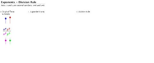
This example dynamically demonstrates the division rule of exponents, visually showing the process of subtracting exponents when the base is the same. It involves core math concepts like exponent operations, function graph transformations, and analytical geometry. GeoGebra commands and objects such as Text, If, Sequence, Segment, Translate, Polygon are used to create step-by-step visualizations and interactive verifications. Suitable for high school mathematics teaching to help students understand and master exponent rules, enhancing mathematical visualization skills.
GeoGebra Commands & Parameters
Text("y") → text4Text("y") → text6Text("x") → text5Text(expX1 + "") → text8Text(expX2 + "") → text9Text(expY1 + "") → text10Text(expY2 + "") → text11Text("________________") → origFracLineIf(color, 255, 0) → factorColor255If(color, 153, 0) → factorColor153Text("x") → text3Text("________________") → fracLineText(abs(expX1 - expX2) + "") → fracXbotYbotExpText(abs(expY1 - expY2) + "") → fracYbotXbotExpText(expY1 - expY2 + "") → fracYtopXbotExpText(abs(expX1 - expX2) + "") → fracXbotYtopExpIf(expX1 - expX2 ≟ 0 ∧ expY1 - expY2 ≟ 0, 1, 0) → zerosText(expX1 - expX2 + "") → fracXtopYtopExpText(abs(expY1 - expY2) + "") → fracYbotXtopExpText(expX1 - expX2 + "") → fracXtopYbotExpText(expY1 - expY2 + "") → fracYtopXtopExpSequence(Translate[xtop, Vector[(0, 0), (((-0.75) * i), 0)]], i, 0, expX1 - 1) → ExpandXtopSequence(Translate[ytop, Vector[(0, 0), ((0.75 * i), 0)]], i, 0, expY1 - 1) → ExpandYtopSequence(Translate[xtop, Vector[(0, 0), (((-0.75) * i), (-1.2))]], i, 0, expX2 - 1) → ExpandXbotSequence(Translate[ytop, Vector[(0, 0), ((0.75 * i), (-1.2))]], i, 0, expY2 - 1) → ExpandYbotSegment((7.5 - (0.75 * If[expX1 > expX2, expX1, expX2]), (-0.5)), (7.5 + (0.75 * If[expY1 > expY2, expY1, expY2]), (-0.5))) → ExpandDivLineTranslate((6.923609046978582, -1.782455570499752), Vector[(0, 0), (0, -3)]) → ATranslate((6.923609046978582, 0.217544429500248), Vector[(0, 0), (0, -3)]) → BTranslate((7.524258469913336, 0.217544429500248), Vector[(0, 0), (0, -3)]) → CTranslate((7.524258469913336, -1.782455570499752), Vector[(0, 0), (0, -3)]) → DPolygon(A, B, C, D) → ShadeNotePoly, a_1, b_1, c_1, d_1Sequence(Polygon[Translate[(6.923609046978582, -1.782455570499752), Vector[(0, 0), (((-0.73) * i), 0)]], Translate[(6.923609046978582, 0.4), Vector[(0, 0), (((-0.73) * i), 0)]], Translate[(7.524258469913336, 0.4), Vector[(0, 0), (((-0.73) * i), 0)]], Translate[(7.524258469913336, -1.782455570499752), Vector[(0, 0), (((-0.73) * i), 0)]]], i, 0, If[expX1 > expX2, expX2, expX1] - 1) → ExpandXPairsSeqSequence(Polygon[Translate[(6.923609046978582, -1.782455570499752), Vector[(0, 0), ((0.73 * i), 0)]], Translate[(6.923609046978582, 0.4), Vector[(0, 0), ((0.73 * i), 0)]], Translate[(7.524258469913336, 0.4), Vector[(0, 0), ((0.73 * i), 0)]], Translate[(7.524258469913336, -1.782455570499752), Vector[(0, 0), ((0.73 * i), 0)]]], i, 1, If[expY1 > expY2, expY2, expY1]) → ExpandYPairsSeq
AI Drawing Prompt Reference
Create a dynamic visualization showing the division rule of exponents, visually demonstrating the process of subtracting exponents when the base is the same. Include function graphs, a slider to control variables, text annotations for exponents and operations, and vector visualizations for exponent changes. Use polygons and segment lines to assist in explaining the process. Start with the basic framework, then dynamically generate visualizations of exponent changes based on slider values, and finally emphasize the result with polygons and segment lines.
The prompt above was compiled from the original drawing commands and is for reference only.