
Exponents: Division Rule Demo
Loading the math board and drawing, please wait…
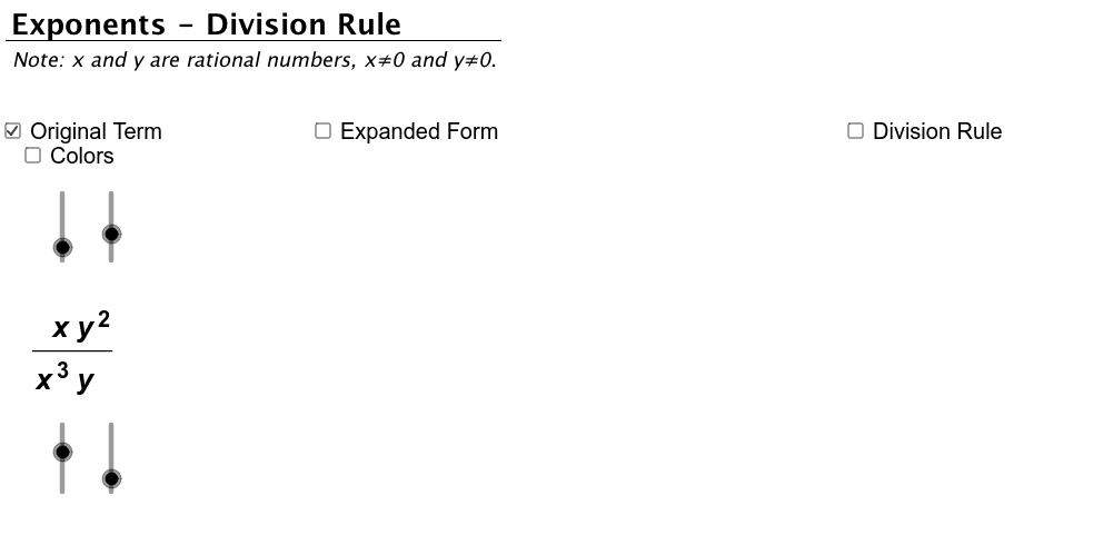
This example demonstrates the geometric representation and calculation process of the exponent division rule. It involves core math concepts like exponent operations, fraction simplification, and geometric transformations. Constructed using GeoGebra commands like Text, If, Sequence, Segment, Translate, Polygon, it provides dynamic graphics and textual explanations. Suitable for high school mathematics teaching and learning, helping to understand exponent properties and geometric intuition.
GeoGebra Commands & Parameters
Text("y") → text4Text("y") → text6Text("x") → text5Text(expX1 + "") → text8Text(expX2 + "") → text9Text(expY1 + "") → text10Text(expY2 + "") → text11Text("________________") → origFracLineIf(color, 255.0, 0.0) → factorColor255If(color, 153.0, 0.0) → factorColor153Text("x") → text3Text("________________") → fracLineText(abs(expX1 - expX2) + "") → fracXbotYbotExpText(abs(expY1 - expY2) + "") → fracYbotXbotExpText(expY1 - expY2 + "") → fracYtopXbotExpText(abs(expX1 - expX2) + "") → fracXbotYtopExpIf(expX1 - expX2 ≟ 0.0 ∧ expY1 - expY2 ≟ 0.0, 1.0, 0.0) → zerosText(expX1 - expX2 + "") → fracXtopYtopExpText(abs(expY1 - expY2) + "") → fracYbotXtopExpText(expX1 - expX2 + "") → fracXtopYbotExpText(expY1 - expY2 + "") → fracYtopXtopExpSequence(Translate[xtop, Vector[(0.0, 0.0), (-(0.75) * i, 0.0)]], i, 0.0, expX1 - 1.0) → ExpandXtopSequence(Translate[ytop, Vector[(0.0, 0.0), (0.75 * i, 0.0)]], i, 0.0, expY1 - 1.0) → ExpandYtopSequence(Translate[xtop, Vector[(0.0, 0.0), (-(0.75) * i, -(1.2))]], i, 0.0, expX2 - 1.0) → ExpandXbotSequence(Translate[ytop, Vector[(0.0, 0.0), (0.75 * i, -(1.2))]], i, 0.0, expY2 - 1.0) → ExpandYbotSegment((7.5 - 0.75 * If[expX1 > expX2, expX1, expX2], -(0.5)), (7.5 + 0.75 * If[expY1 > expY2, expY1, expY2], -(0.5))) → ExpandDivLineTranslate((6.923609046978582, -1.782455570499752), Vector[Vector[(0.0, 0.0), (0.0, -3.0)]]) → ATranslate((6.923609046978582, 0.217544429500248), Vector[Vector[(0.0, 0.0), (0.0, -3.0)]]) → BTranslate((7.524258469913336, 0.217544429500248), Vector[Vector[(0.0, 0.0), (0.0, -3.0)]]) → CTranslate((7.524258469913336, -1.782455570499752), Vector[Vector[(0.0, 0.0), (0.0, -3.0)]]) → DPolygon(A, B, C, D) → ShadeNotePoly, a_1, b_1, c_1, d_1Sequence(Polygon[Translate[(6.923609046978582, -1.782455570499752), Vector[(0.0, 0.0), (-(0.73) * i, 0.0)]], Translate[(6.923609046978582, 0.4), Vector[(0.0, 0.0), (-(0.73) * i, 0.0)]], Translate[(7.524258469913336, 0.4), Vector[(0.0, 0.0), (-(0.73) * i, 0.0)]], Translate[(7.524258469913336, -1.782455570499752), Vector[(0.0, 0.0), (-(0.73) * i, 0.0)]]], i, 0.0, If[expX1 > expX2, expX2, expX1] - 1.0) → ExpandXPairsSeqSequence(Polygon[Translate[(6.923609046978582, -1.782455570499752), Vector[(0.0, 0.0), (0.73 * i, 0.0)]], Translate[(6.923609046978582, 0.4), Vector[(0.0, 0.0), (0.73 * i, 0.0)]], Translate[(7.524258469913336, 0.4), Vector[(0.0, 0.0), (0.73 * i, 0.0)]], Translate[(7.524258469913336, -1.782455570499752), Vector[(0.0, 0.0), (0.73 * i, 0.0)]]], i, 1.0, If[expY1 > expY2, expY2, expY1]) → ExpandYPairsSeq
AI Drawing Prompt Reference
Create a geometric illustration demonstrating the exponent division rule, showing two exponent expressions and their division in fraction form, along with geometric transformations. Start by drawing the two exponent expressions and labeling their values, then connect them with a fraction bar. Use geometric transformations (translations and scalings) to visualize the result of the exponent division, emphasizing the geometric meaning with polygons and lines.
The prompt above was compiled from the original drawing commands and is for reference only.