
Exponent Problem Demonstration
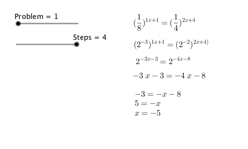
Loading the math board and drawing, please wait…
In collections
Exponents
This example demonstrates the graph and properties of exponential functions, dynamically showcasing exponential growth and decay phenomena. Core math concepts include exponent operations, median value, bar charts, optimization problems, polynomial functions, and variance analysis. Construction highlights involve GeoGebra commands like RandomElement, Element, If, and objects A1-D10 for data generation and conditional logic. Suitable for high school mathematics teaching, focusing on exponential function applications and data analysis.
GeoGebra Commands & Parameters
RandomElement({2, 3, 5}) → A1RandomElement({2, 3, 5}) → A2RandomElement({2, 3, 5}) → A3RandomElement({2, 3, 5}) → A4RandomElement({2, 3, 5}) → A5RandomElement({2, 3, 5}) → A6RandomElement({2, 3, 5}) → A7RandomElement({2, 3, 5}) → A8RandomElement({2, 3, 5}) → A9RandomElement({2, 3, 5}) → A10RandomElement({-4, -3, -2, -1, 2, 3, 4}) → B1RandomElement({-4, -3, -2, -1, 2, 3, 4}) → B2RandomElement({-4, -3, -2, -1, 2, 3, 4}) → B3RandomElement({-4, -3, -2, -1, 2, 3, 4}) → B4RandomElement({-4, -3, -2, -1, 2, 3, 4}) → B5RandomElement({-4, -3, -2, -1, 2, 3, 4}) → B6RandomElement({-4, -3, -2, -1, 2, 3, 4}) → B7RandomElement({-4, -3, -2, -1, 2, 3, 4}) → B8RandomElement({-4, -3, -2, -1, 2, 3, 4}) → B9RandomElement({-4, -3, -2, -1, 2, 3, 4}) → B10RandomElement({-3, -2, -1, 1, 2, 3, 4}) → C1RandomElement({-3, -2, -1, 1, 2, 3, 4}) → C2RandomElement({-3, -2, -1, 1, 2, 3, 4}) → C3RandomElement({-3, -2, -1, 1, 2, 3, 4}) → C4RandomElement({-3, -2, -1, 1, 2, 3, 4}) → C5RandomElement({-3, -2, -1, 1, 2, 3, 4}) → C6RandomElement({-3, -2, -1, 1, 2, 3, 4}) → C7RandomElement({-3, -2, -1, 1, 2, 3, 4}) → C8RandomElement({-3, -2, -1, 1, 2, 3, 4}) → C9RandomElement({-3, -2, -1, 1, 2, 3, 4}) → C10RandomElement({-3, -2, -1, 1, 2, 3, 4}) → D1RandomElement({-3, -2, -1, 1, 2, 3, 4}) → D2RandomElement({-3, -2, -1, 1, 2, 3, 4}) → D3RandomElement({-3, -2, -1, 1, 2, 3, 4}) → D4RandomElement({-3, -2, -1, 1, 2, 3, 4}) → D5RandomElement({-3, -2, -1, 1, 2, 3, 4}) → D6RandomElement({-3, -2, -1, 1, 2, 3, 4}) → D7RandomElement({-3, -2, -1, 1, 2, 3, 4}) → D8RandomElement({-3, -2, -1, 1, 2, 3, 4}) → D9RandomElement({-3, -2, -1, 1, 2, 3, 4}) → D10RandomElement({-3, -2, -1, 1, 2, 3, 4}) → E1RandomElement({-3, -2, -1, 1, 2, 3, 4}) → F1RandomElement({-3, -2, -1, 1, 2, 3, 4}) → E2RandomElement({-3, -2, -1, 1, 2, 3, 4}) → F2RandomElement({-3, -2, -1, 1, 2, 3, 4}) → E3RandomElement({-3, -2, -1, 1, 2, 3, 4}) → F3RandomElement({-3, -2, -1, 1, 2, 3, 4}) → E4RandomElement({-3, -2, -1, 1, 2, 3, 4}) → F4RandomElement({-3, -2, -1, 1, 2, 3, 4}) → E5RandomElement({-3, -2, -1, 1, 2, 3, 4}) → F5RandomElement({-3, -2, -1, 1, 2, 3, 4}) → E6RandomElement({-3, -2, -1, 1, 2, 3, 4}) → F6RandomElement({-3, -2, -1, 1, 2, 3, 4}) → E7RandomElement({-3, -2, -1, 1, 2, 3, 4}) → F7RandomElement({-3, -2, -1, 1, 2, 3, 4}) → E8RandomElement({-3, -2, -1, 1, 2, 3, 4}) → F8RandomElement({-3, -2, -1, 1, 2, 3, 4}) → E9RandomElement({-3, -2, -1, 1, 2, 3, 4}) → F9RandomElement({-3, -2, -1, 1, 2, 3, 4}) → E10RandomElement({-3, -2, -1, 1, 2, 3, 4}) → F10RandomElement({-4, -3, -2, -1, 2, 3, 4}) → I1RandomElement({-4, -3, -2, -1, 2, 3, 4}) → I2RandomElement({-4, -3, -2, -1, 2, 3, 4}) → I3RandomElement({-4, -3, -2, -1, 2, 3, 4}) → I4RandomElement({-4, -3, -2, -1, 2, 3, 4}) → I5RandomElement({-4, -3, -2, -1, 2, 3, 4}) → I6RandomElement({-4, -3, -2, -1, 2, 3, 4}) → I7RandomElement({-4, -3, -2, -1, 2, 3, 4}) → I8RandomElement({-4, -3, -2, -1, 2, 3, 4}) → I9RandomElement({-4, -3, -2, -1, 2, 3, 4}) → I10Element(A1:A10, Problem) → baseElement(B1:B10, Problem) → baseexp1Element(I1:I10, Problem) → baseexp2Element(G1:G10, Problem) → exp1Element(H1:H10, Problem) → exp2If(Defined[sol], true, false) → a
AI Drawing Prompt Reference
Create a dynamic graph demonstrating exponential growth and decay, featuring randomly generated data points, multiple exponential curves in different colors, key points like median and variance marked, bar charts showing probability distribution, and optimized curves to highlight function properties.
The prompt above was compiled from the original drawing commands and is for reference only.