
Exploring Numerical Integration
Loading the math board and drawing, please wait…
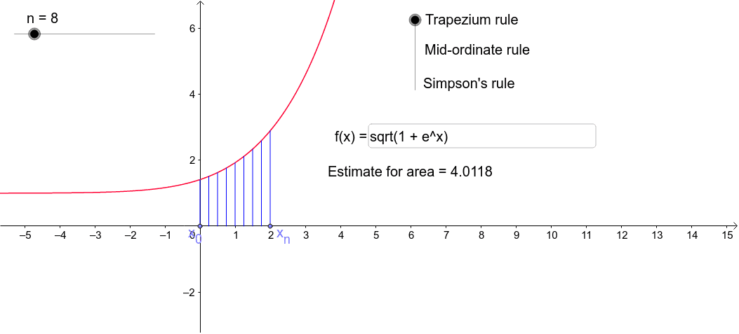
This applet explores three methods of numerical integration: trapezoidal, Simpson's, and rectangular methods. It helps students understand the concept of integration by observing the approximation effects with different step sizes. The applet uses commands like Point, If, Sequence, Element, etc., suitable for high school mathematics education.
GeoGebra Commands & Parameters
Point(xAxis) → x_nPoint(xAxis) → x_0If(c ≟ 0 ∧ IsInteger[(n + 1) / 2], 1, 0) → zIf(z ≟ 0, n) → n_2If(c ≟ 0, d_1, d) → d_2Sequence((i, 0), i, a, b, d_2) → LElement(L, A2) → B1Element(L, A3) → B2Element(L, A4) → B3Element(L, A13) → B12Element(L, A12) → B11Element(L, A11) → B10OrthogonalLine(x_0, xAxis) → pOrthogonalLine(x_n, xAxis) → qElement(L, A5) → B4Element(L, A6) → B5Element(L, A7) → B6Element(L, A8) → B7Element(L, A9) → B8Element(L, A10) → B9Element(L, A14) → B13Element(L, A15) → B14Element(L, A16) → B15Element(L, A17) → B16Element(L, A18) → B17Element(L, A19) → B18Element(L, A20) → B19Element(L, A21) → B20Element(L, A22) → B21Element(L, A23) → B22Element(L, A24) → B23Element(L, A25) → B24Element(L, A26) → B25Element(L, A27) → B26Element(L, A28) → B27Element(L, A29) → B28Element(L, A30) → B29Element(L, A31) → B30Element(L, A32) → B31Element(L, A33) → B32Element(L, A34) → B33Element(L, A35) → B34Element(L, A36) → B35Element(L, A37) → B36Element(L, A38) → B37Element(L, A39) → B38Element(L, A40) → B39Element(L, A41) → B40Element(L, A42) → B41Element(L, A43) → B42Element(L, A44) → B43Element(L, A45) → B44Element(L, A46) → B45Element(L, A47) → B46Element(L, A48) → B47Element(L, A49) → B48Element(L, A50) → B49Segment(B1, (x(B1), f(x(B1)))) → C1Segment(B2, (x(B2), f(x(B2)))) → C2Segment(B3, (x(B3), f(x(B3)))) → C3Segment(B4, (x(B4), f(x(B4)))) → C4Segment(B5, (x(B5), f(x(B5)))) → C5Segment(B6, (x(B6), f(x(B6)))) → C6Segment(B7, (x(B7), f(x(B7)))) → C7Segment(B8, (x(B8), f(x(B8)))) → C8Segment(B9, (x(B9), f(x(B9)))) → C9Segment(B10, (x(B10), f(x(B10)))) → C10Segment(B11, (x(B11), f(x(B11)))) → C11Segment(B12, (x(B12), f(x(B12)))) → C12Segment(B13, (x(B13), f(x(B13)))) → C13Segment(B14, (x(B14), f(x(B14)))) → C14Segment(B15, (x(B15), f(x(B15)))) → C15Segment(B16, (x(B16), f(x(B16)))) → C16Segment(B17, (x(B17), f(x(B17)))) → C17Segment(B18, (x(B18), f(x(B18)))) → C18Segment(B19, (x(B19), f(x(B19)))) → C19Segment(B20, (x(B20), f(x(B20)))) → C20Segment(B21, (x(B21), f(x(B21)))) → C21Segment(B22, (x(B22), f(x(B22)))) → C22Segment(B23, (x(B23), f(x(B23)))) → C23Segment(B24, (x(B24), f(x(B24)))) → C24Segment(B25, (x(B25), f(x(B25)))) → C25Segment(B26, (x(B26), f(x(B26)))) → C26Segment(B27, (x(B27), f(x(B27)))) → C27Segment(B28, (x(B28), f(x(B28)))) → C28Segment(B29, (x(B29), f(x(B29)))) → C29Segment(B30, (x(B30), f(x(B30)))) → C30Segment(B31, (x(B31), f(x(B31)))) → C31Segment(B32, (x(B32), f(x(B32)))) → C32Segment(B33, (x(B33), f(x(B33)))) → C33Segment(B34, (x(B34), f(x(B34)))) → C34Segment(B35, (x(B35), f(x(B35)))) → C35Segment(B36, (x(B36), f(x(B36)))) → C36Segment(B37, (x(B37), f(x(B37)))) → C37Segment(B38, (x(B38), f(x(B38)))) → C38Segment(B39, (x(B39), f(x(B39)))) → C39Segment(B40, (x(B40), f(x(B40)))) → C40Segment(B41, (x(B41), f(x(B41)))) → C41Segment(B42, (x(B42), f(x(B42)))) → C42Segment(B43, (x(B43), f(x(B43)))) → C43Segment(B44, (x(B44), f(x(B44)))) → C44Segment(B45, (x(B45), f(x(B45)))) → C45Segment(B46, (x(B46), f(x(B46)))) → C46Segment(B47, (x(B47), f(x(B47)))) → C47Segment(B48, (x(B48), f(x(B48)))) → C48Segment(B49, (x(B49), f(x(B49)))) → C49Sum(RemoveUndefined[L_1]) → tSum(RemoveUndefined[L_2]) → mIf(IsInteger[(A1 + 1) / 2], F1, 0) → G1If(IsInteger[(A2 + 1) / 2], F2, 0) → G2If(IsInteger[(A3 + 1) / 2], F3, 0) → G3If(IsInteger[(A4 + 1) / 2], F4, 0) → G4If(IsInteger[(A5 + 1) / 2], F5, 0) → G5If(IsInteger[(A6 + 1) / 2], F6, 0) → G6If(IsInteger[(A7 + 1) / 2], F7, 0) → G7If(IsInteger[(A8 + 1) / 2], F8, 0) → G8If(IsInteger[(A9 + 1) / 2], F9, 0) → G9If(IsInteger[(A10 + 1) / 2], F10, 0) → G10If(IsInteger[(A11 + 1) / 2], F11, 0) → G11If(IsInteger[(A12 + 1) / 2], F12, 0) → G12If(IsInteger[(A13 + 1) / 2], F13, 0) → G13If(IsInteger[(A14 + 1) / 2], F14, 0) → G14If(IsInteger[(A15 + 1) / 2], F15, 0) → G15If(IsInteger[(A16 + 1) / 2], F16, 0) → G16If(IsInteger[(A17 + 1) / 2], F17, 0) → G17If(IsInteger[(A18 + 1) / 2], F18, 0) → G18If(IsInteger[(A19 + 1) / 2], F19, 0) → G19If(IsInteger[(A20 + 1) / 2], F20, 0) → G20If(IsInteger[(A21 + 1) / 2], F21, 0) → G21If(IsInteger[(A22 + 1) / 2], F22, 0) → G22If(IsInteger[(A23 + 1) / 2], F23, 0) → G23If(IsInteger[(A24 + 1) / 2], F24, 0) → G24If(IsInteger[(A25 + 1) / 2], F25, 0) → G25If(IsInteger[(A26 + 1) / 2], F26, 0) → G26If(IsInteger[(A27 + 1) / 2], F27, 0) → G27If(IsInteger[(A28 + 1) / 2], F28, 0) → G28If(IsInteger[(A29 + 1) / 2], F29, 0) → G29If(IsInteger[(A30 + 1) / 2], F30, 0) → G30If(IsInteger[(A31 + 1) / 2], F31, 0) → G31If(IsInteger[(A32 + 1) / 2], F32, 0) → G32If(IsInteger[(A33 + 1) / 2], F33, 0) → G33If(IsInteger[(A34 + 1) / 2], F34, 0) → G34If(IsInteger[(A35 + 1) / 2], F35, 0) → G35If(IsInteger[(A36 + 1) / 2], F36, 0) → G36If(IsInteger[(A37 + 1) / 2], F37, 0) → G37If(IsInteger[(A38 + 1) / 2], F38, 0) → G38If(IsInteger[(A39 + 1) / 2], F39, 0) → G39If(IsInteger[(A40 + 1) / 2], F40, 0) → G40If(IsInteger[(A41 + 1) / 2], F41, 0) → G41If(IsInteger[(A42 + 1) / 2], F42, 0) → G42If(IsInteger[(A43 + 1) / 2], F43, 0) → G43If(IsInteger[(A44 + 1) / 2], F44, 0) → G44If(IsInteger[(A45 + 1) / 2], F45, 0) → G45If(IsInteger[(A46 + 1) / 2], F46, 0) → G46If(IsInteger[(A47 + 1) / 2], F47, 0) → G47If(IsInteger[(A48 + 1) / 2], F48, 0) → G48Sum(RemoveUndefined[L_3]) → sElement(L, A51) → B50Element(L, A52) → B51Segment(B50, (x(B50), f(x(B50)))) → C50Segment(B51, (x(B51), f(x(B51)))) → C51If(IsInteger[(A49 + 1) / 2], F49, 0) → G49If(IsInteger[(A50 + 1) / 2], F50, 0) → G50Textfield(f) → inputBox1
AI Drawing Prompt Reference
Draw a function graph and display three numerical integration methods: trapezoidal, Simpson's, and rectangular. Use a slider to adjust the step size and observe the approximation effects of integration under different step sizes. Mark multiple points on the x-axis and connect them to the function graph with orthogonal lines to form the integration area.
The prompt above was compiled from the original drawing commands and is for reference only.