
Binomial Distribution Hypothesis Testing
Loading the math board and drawing, please wait…
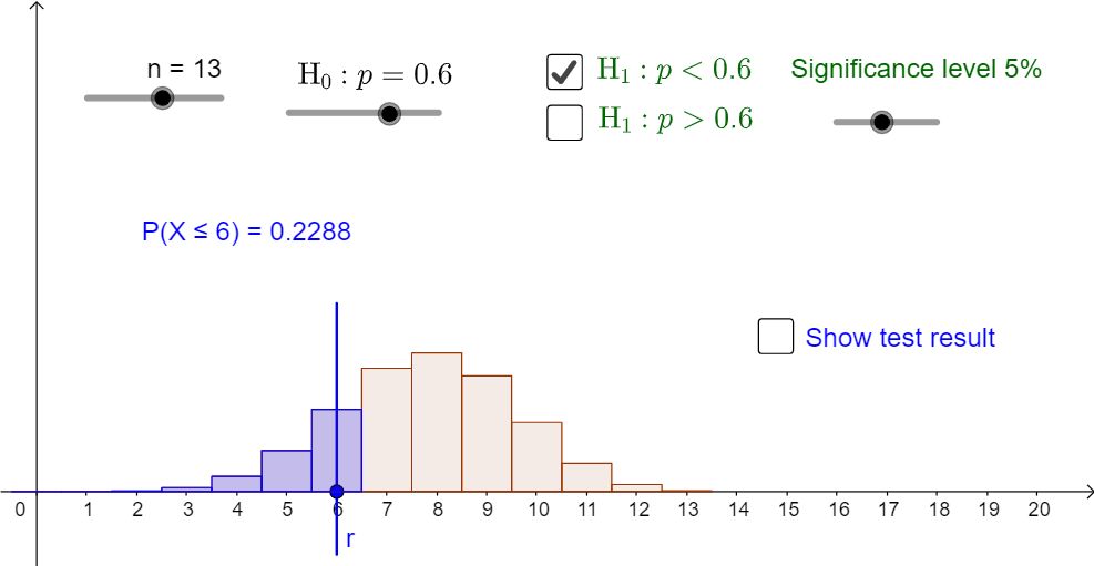
This example demonstrates hypothesis testing using the binomial distribution, visualizing the comparison between sample data and theoretical distribution. Core math concepts include binomial distribution, hypothesis testing, p-value, critical value. GeoGebra commands used are Sequence, BarChart, Element, Segment, Point, If, with objects like p, n, L, e, s, text12, a, S, c_1, c_2, c_4, sig_1, sig_2, c_3, s_3, s_4, A, B, i, X, j, k, x_1, text9, l, x_2, text10, text11, s_1, s_2, m, text2, text3_1, text4, o, q, text13. Suitable for high school and above learners to understand statistical inference and binomial distribution applications.
GeoGebra Commands & Parameters
Sequence(((nCr[n, r] * p^(r)) * (1 - p)^(n - r)), r, 0, n) → L, {0.000006710886400000005, 0.00013086228480000008, 0.0011777605632000007, 0.0064776830976000024, 0.02429131161600001, 0.06558654136320002, 0.13117308272640002, 0.19675962408960004, 0.22135457710079995, 0.18446214758399998, 0.11067728855039997, 0.04527707258879999, 0.011319268147199996, 0.0013060694015999993}BarChart(-0.5, n + 0.5, L) → aSequence(Sum[L, i], i, 1, n + 1) → SElement(S, c_3 + 1) → s_3Segment(A, B) → iPoint(i) → XSegment((x(X), 0.3), (x(X), -0.1)) → jBarChart(-0.5, x(X) + 0.5, Take[L, 1, x(X) + 1]) → kElement(S, x(X) + 1) → x_1BarChart(x(X) - 0.5, n + 0.5, Take[L, x(X) + 1, n + 1]) → lIf(x(X) > 0, 1 - Element[S, x(X)], 1) → x_2Element(S, c_1 + 1) → s_1
AI Drawing Prompt Reference
Create a visualization for binomial distribution hypothesis testing, featuring a bar chart for the theoretical distribution, another for sample data, and a point indicating the current sample position. A vertical segment extends from the point, with two segments below connecting to the corresponding bars in the sample and theoretical distributions. The bars to the left and right of the point represent the theoretical distribution before and after the current sample position, respectively. Display the cumulative probability value of the current sample above the point.
The prompt above was compiled from the original drawing commands and is for reference only.