
Hypothesis Testing with Binomial Distribution
Loading the math board and drawing, please wait…
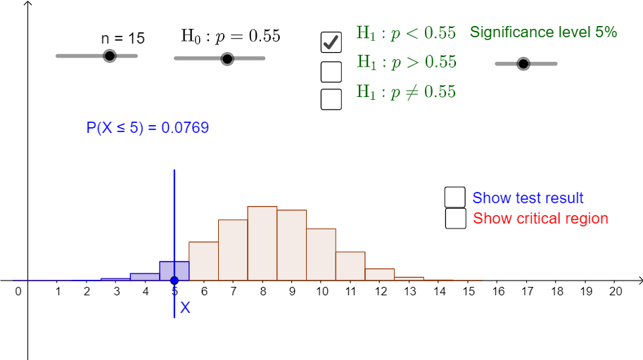
This example demonstrates the statistical process of hypothesis testing using the binomial distribution. Key math concepts include probability & statistics, hypothesis testing, and the binomial distribution. Construction highlights involve GeoGebra commands/objects like Sequence, BarChart, Element, Segment, Point, and If. Suitable for high school and above students learning statistical inference methods.
GeoGebra Commands & Parameters
Sequence(((nCr[n, r] * p^(r)) * (1 - p)^(n - r)), r, 0, n) → LBarChart(-0.5, n + 0.5, L) → aSequence(Sum[L, i], i, 1, n + 1) → SBarChart(-0.5, c_1 + 0.5, Take[L, 1, c_1 + 1]) → cBarChart(c_2 - 0.5, n + 0.5, Take[L, c_2 + 1, n + 1]) → dBarChart(-0.5, c_3 + 0.5, Take[L, 1, c_3 + 1]) → fElement(S, c_3 + 1) → s_3BarChart(c_4 - 0.5, n + 0.5, Take[L, c_4 + 1, n + 1]) → gSegment(A, B) → iPoint(i) → XSegment((x(X), 0.3), (x(X), -0.1)) → jBarChart(-0.5, x(X) + 0.5, Take[L, 1, x(X) + 1]) → kElement(S, x(X) + 1) → x_1BarChart(x(X) - 0.5, n + 0.5, Take[L, x(X) + 1, n + 1]) → lIf(x(X) > 0, 1 - Element[S, x(X)], 1) → x_2Element(S, c_1 + 1) → s_1
AI Drawing Prompt Reference
Illustrate the hypothesis testing process with a binomial distribution, featuring probability and statistics charts controlled by a slider, showing distributions under different probabilities with bar charts, and marking key data points with points and line segments. Start by drawing the overall distribution, then highlight specific intervals and critical values, and finally connect points with lines to represent the testing process.
The prompt above was compiled from the original drawing commands and is for reference only.