
Exploring Mean and Standard Deviation (Updated)
Loading the math board and drawing, please wait…
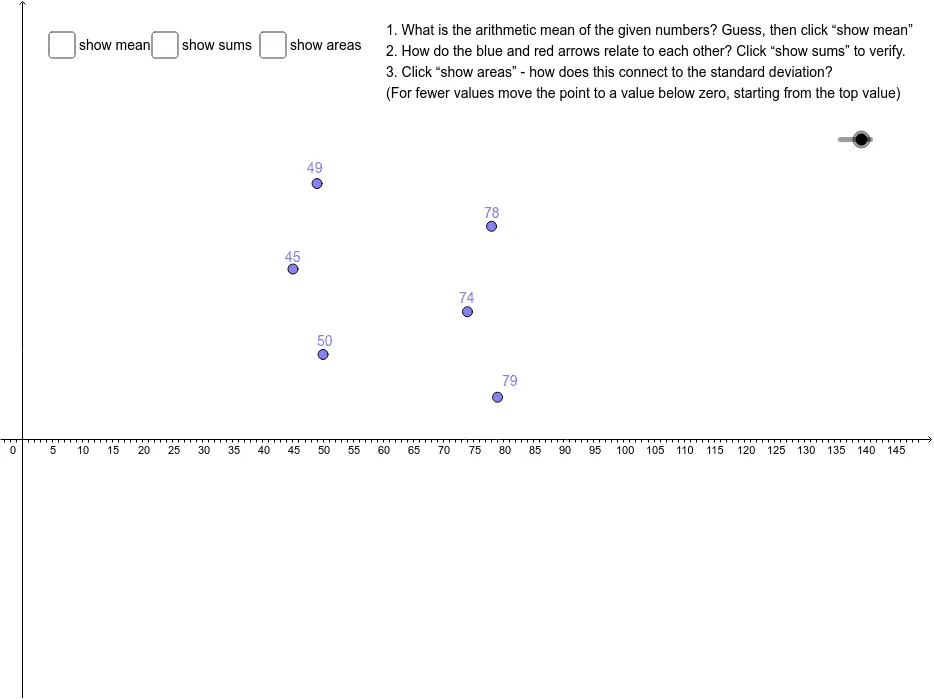
① This interactive GeoGebra example dynamically demonstrates how the mean and standard deviation of a dataset change as data points are moved, with visual representation of the standard deviation interval. ② Core mathematical concepts include arithmetic mean, standard deviation as a measure of dispersion, data distribution visualization, and the role of standard deviation in hypothesis testing. ③ Construction highlights: using GeoGebra commands such as Point to create data points, Mean and Sum for statistical calculations, Vector and Polygon to draw the mean line and standard deviation bands, Circle to illustrate distances, and If/RemoveUndefined for conditional display; objects include multiple points, segments, polygons, and sliders (e.g., sc, g, B) that allow real-time manipulation. ④ Suitable for middle school statistics and probability, as well as introductory college statistics courses, to build intuition about descriptive statistics and support early hypothesis testing demonstrations.
GeoGebra Commands & Parameters
Point(g) → BIf(x(B) ≥ 0, x(B)) → bPoint(k) → FIf(x(F) ≥ 0, x(F)) → fPoint(j) → EIf(x(E) ≥ 0, x(E)) → ePoint(i) → DIf(x(D) ≥ 0, x(D)) → dPoint(h) → CIf(x(C) ≥ 0, x(C)) → cPoint(l) → AIf(x(A) ≥ 0, x(A)) → aRemoveUndefined(L_2) → L_1Mean(L_1) → mIf(A1 - m < 0, 1, 0) → B1Mean({a, b, c, d, e, f}) → vIf(A1 - m > 0, 1, 0) → C1If(A2 - m < 0, 1, 0) → B2If(A3 - m < 0, 1, 0) → B3If(A4 - m < 0, 1, 0) → B4If(A5 - m < 0, 1, 0) → B5If(A6 - m < 0, 1, 0) → B6If(A2 - m > 0, 1, 0) → C2If(A3 - m > 0, 1, 0) → C3If(A4 - m > 0, 1, 0) → C4If(A5 - m > 0, 1, 0) → C5If(A6 - m > 0, 1, 0) → C6Sum(D1:D6) → D7Sum(E1:E6) → E7Vector((m, 0), (m - D9, 0)) → D16Vector((m, 0), (m - D10, 0)) → D17Vector((m, 0), (m - D11, 0)) → D18Vector((m, 0), (m - D12, 0)) → D19Vector((m, 0), (m - D13, 0)) → D20Vector((m, 0), (m - D14, 0)) → D21Vector((m, 0), (m + E9, 0)) → E16Vector((m, 0), (m + E10, 0)) → E17Vector((m, 0), (m + E11, 0)) → E18Vector((m, 0), (m + E12, 0)) → E19Vector((m, 0), (m + E13, 0)) → E20Vector((m, 0), (m + E14, 0)) → E21Vector((m, (5 * sc)), (x(E), (5 * sc))) → nVector((m, (4 * sc)), (x(D), (4 * sc))) → pVector((m, (3 * sc)), (x(C), (3 * sc))) → qVector((m, (2 * sc)), (x(B), (2 * sc))) → rVector((m, sc), (x(A), sc)) → sVector((m, (6 * sc)), (x(F), (6 * sc))) → wPolygon(C15, C16, (x(C16), (-D1)), (x(C15), (-D1))) → B16, t, f_1, g_1, h_1Vector((m, 0), (m, (7 * sc))) → uPolygon(C16, C17, (x(C17), (-D2)), (x(C16), (-D2))) → B17, i_1, j_1, k_1, l_1Polygon(C17, C18, (x(C18), (-D3)), (x(C17), (-D3))) → B18, m_1, n_1, p_1, q_1Polygon(C18, C19, (x(C19), (-D4)), (x(C18), (-D4))) → B19, r_1, s_1, t_1, a_1Polygon(C19, C20, (x(C20), (-D5)), (x(C19), (-D5))) → B20, b_1, c_1, d_1, e_1Polygon(C20, C21, (x(C21), (-D6)), (x(C20), (-D6))) → B21, f_2, g_2, h_2, i_2Polygon(F15, F16, (x(F16), (-E1)), (x(F15), (-E1))) → G16, H16_1, I16, J16, K16Polygon(F16, F17, (x(F17), (-E2)), (x(F16), (-E2))) → G17, H17_1, I17, J17, K17Polygon(F17, F18, (x(F18), (-E3)), (x(F17), (-E3))) → G18, H18_1, I18, J18, K18Polygon(F18, F19, (x(F19), (-E4)), (x(F18), (-E4))) → G19, H19_1, I19, J19, K19Polygon(F19, F20, (x(F20), (-E5)), (x(F19), (-E5))) → G20, H20_1, I20, J20, K20Polygon(F20, F21, (x(F21), (-E6)), (x(F20), (-E6))) → G21, H21_1, I21, J21, K21Circle((m, 0), D7) → c_2
AI Drawing Prompt Reference
Draw six draggable data points on a coordinate plane, keeping only their non-negative x-coordinates. Compute their mean and display a vertical line at the mean. From the mean line, draw horizontal vectors to each point to show deviations. Shade the standard deviation interval on both sides of the mean with semi-transparent polygons. Above the mean line, at different heights, draw horizontal segments connecting the mean to each point's x-coordinate to visualize distances. Include sliders to adjust the standard deviation scaling and update all graphics in real time.
The prompt above was compiled from the original drawing commands and is for reference only.